For the project deliverable in this class, you will create a “webapp” using streamlit.
The purpose of the “app” will be to provide a tool for fitting curves to data. The interface should include:
A way for users to enter data (x and y values). This should include:
A data entry area for users to enter data by hand
An option to upload data in the form of a CSV file
The ability to fit multiple different types of curves, such as polynomials, statistical distributions, and other miscillaneous types.
It is possible to use the “least-squares” method to fit curves, and there are also buit-in functions for curve fitting in some packages (e.g. polyfit in scipy)
A visualization of the data and the fitted curve (i.e. a graph)
An output area that shows the fitting parameters with some information about the quality of the fit (e.g. average error or maximum error between data and curve)
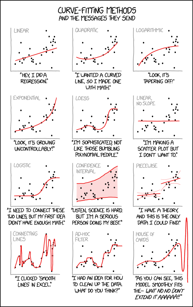
Figure K.1: Some examples of fitting different curves to data. Also some examples of how curve fitting can be used to justify anything.
K.1 Using streamlit
Streamlit is a Python package which provides tools for making a “graphical user interface”. The power of Streamlit is that is uses the interface tools provided by web browsers (think of the upload buttons, date pickers, etc we find on webpages), and renders your app in a browser instead of requiring users to download a (large) application file.
At it simplest, Streamlit works as follows:
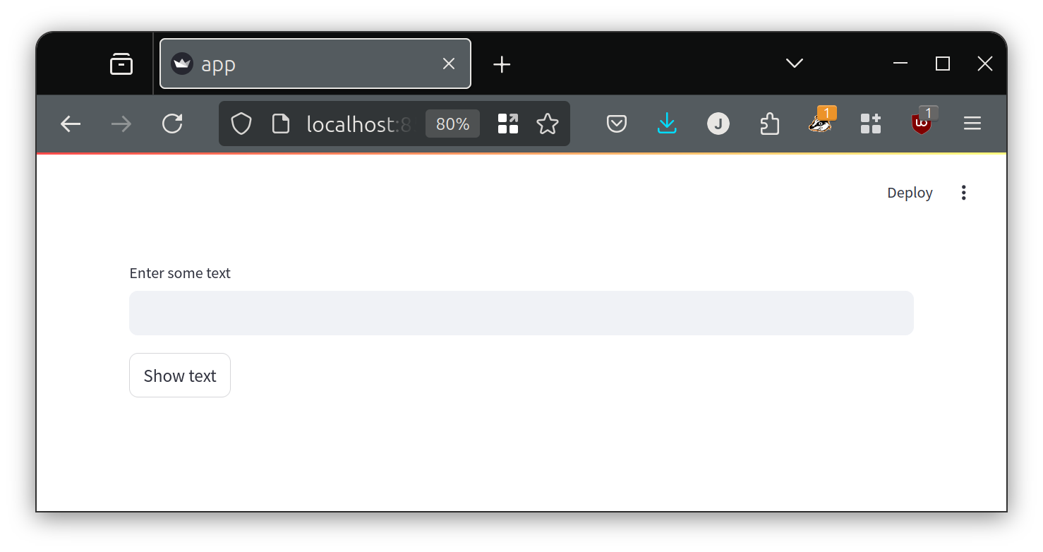
import streamlit as sttext = st.text_input(label='Enter some text')if st.button(label='Show text'): st.write(text)
To actually run this file and start the app, you need to save the above file (e.g. app.py), open your “conda” prompt, and navigate to the folder containing the file. Then type:
(base)C:\<some path>\ streamlit run app.py
This should result in your web browser opening and showing a new tab like the following:
Figure K.2: A screenshot of the Streamlit app described above.
Let’s look at the code again more closely:
import streamlit as st1text = st.text_input(label='Enter some text')2if st.button(label='Show text'):3 st.write(text)
1
This line does two things. Firstly, it creates a Streamlit “text_input” field in the app. Secondly, it tells our python program that the value entered into the field should be stored in text.
2
This line also does two things: Firstly, it creates a Streamlit “button” in the app. Secondly, it provides the True/False value to python for the “If-statement”. Clicking the button sends True.
3
When the button is clicked Streamlit “writes” the value of text to the app.
A main thing to note here is that the elements in the user interface (i.e. textbox, button, output) appear in the same order as in the app.py file. This is how you control the layout of the app.
Streamlit does a lot of the placement for us by default so we don’t have to think about it, which is why it is so easy to use. However, it does limit our creative freedom on the layout.
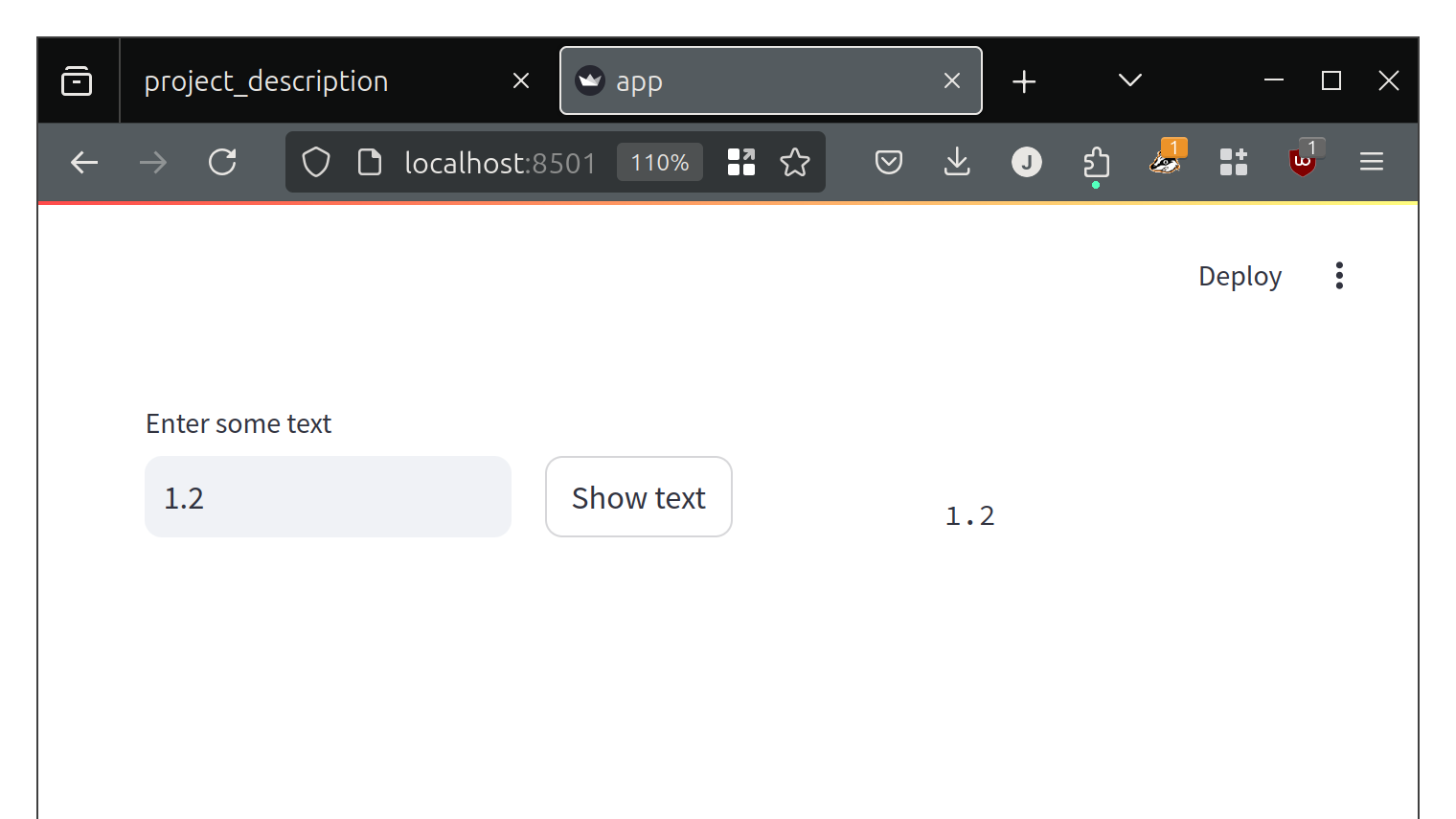
Here is a version of the above app using 3 columns to make the elements all appear on the same line:
import streamlit as st1cols = st.columns(3, vertical_alignment="bottom")2text = cols[0].text_input(label='Enter some text')if cols[1].button(label='Show text'): cols[2].text(text)
1
In this case we have created a set of columns which are located at the top of the page since they are created at the top of the script
2
Note that we can insert elements into any column at point in the script. They will appear on the page in the order we insert them, but we can do it anywhere we look. For instance, we can put cols[0].text('Enter text above') at the bottom of the above script to add text below the text input box.
And here is the result:
Figure K.3: A screenshot of a simple Streamlit app using 3 columns to place elements horizontally.
One of the learning outcomes for this project is that you’ll dig into the documentation and examples on Streamlit to customize your interface.
K.2 Using numpy.polyfit
Numpy
We have not talked about numpy and “ND-arrays” yet, but it turns out that we can use normal Python lists as input to many of the numpy functions, so can proceed without knowing the details. Numpy converts them to “ND-arrays” for us.
One of these many functions is called polyfit, which accepts x data, y data and the desired order of the polynomial, then returns the coefficients of the polynomial that fits the data. For instance, if the order is 3, then the polynomial is:
\[
y = a_0 + a_1x + a_2x^2 + a_3x^3
\]
The polyfit function returns the \(a_n\) values in a tuple. The usage of this function is:
import numpy as np1x = np.linspace(0, 10, 100)2y =4.1*x**3+2.4*x**2-8.5*x +2.23coeffs = np.polyfit(x, y, 3)print(coeffs)
1
Generate 100 evenly spaced x-values between 0 and 10
2
Generate y-values for each x-value using some arbitrary coefficients
3
Here we call the polyfit function.
[ 4.1 2.4 -8.5 2.2]
When we print the coeffs we can see that numpy found the exact same coefficients we used to generate the data!
K.3 Using scipy.optimize.curve_fit
polyfit is great, but only works on one type of equation. What if we want to fit the Arrhenius equation to kinetic data?
\[
k = A e^{-E/RT}
\]
Here the fitting parameters are \(A\) and \(E\), given the \(k\) value at various temperatures, \(T\).
It is possible to fit arbitrary equations using the “method of least squares”. The method works as follows (for the example of the Arrhenius equation):
Using the known values of \(T\), find \(k\) using guessed values of \(E\) and \(A\).
Compute the difference between the true (measured) values of \(k\) and the calculated values from step 1.
Square the errors so they are all positive.
Sum the errors for each data point to get a single value. This gives the method its name.
Guess new values of \(E\) and \(A\) until you get the smallest possible sum in step 4.
Step 5 is actually the hardest part because you don’t know how to guess new values of \(E\) and \(A\).
Luckily, scipy has a solution: scipy.optimize.curve_fit. Let’s see how this works. First let’s generate some fake data:
T = [200, 300, 400, 500]e =2.71828R =8.314k = []for temp in T: k.append(1e-5*e**(-8440/(R*temp)))print(k)
There is one important item to notice here: p0 is the initial guess for the parameters being fit. This not only tells curve_fit where to start, but it also tell curve_fithow many parameters are being fit! So the first value in p0 gets passed to A and the second value is passed to E.
curve_fit returns a tuple of the fitted constants, and the computed y-values (\(k\) in this case).
print(coeffs[0])
[1.00000000e-05 8.43968953e+03]
Amazingly it has nearly exactly recovered the coefficients we used when we generated the fake data!
Using the above code we can see that we need to write a function for each equation we wish to support in our app.