6  Files and IO

Learning objectives for this lesson

Upon completion of this lesson you should:

• …appreciate the 2 main types of memory in a computer
• …be familar with the file system, files, and folders
• …understand both relative and absolute file paths
• …know how to write simple text to a file, and read it back in
• …be able to format text to create desired output in files
• …be able to use the command line to perform basic tasks directly
• …know how to install external python libraries using the command line

Figure 6.1: We should probably know a bit more deeply about how a computer works

6.1 Types of Memory

We have not talked much about how computers work internally. As we write more complicated computer programs we need to understand more about how the computer deals with data because it impacts performance. Examples of this trend are advanced numerical algorithms such as machine learning or climate modeling.

The job of “data scientist” is a relatively new phenomena. It entails not only working with scientific data, but also applying scientific concepts and tools to data. It is considered separate from a software engineer or computer programmer. One of the main considerations when doing data science, and scientific programming in general, is ensuring good performance. Crunching a gazillion data points is only useful if it can be done quickly.

It is convenient to think of computer memory as being either permanent and slow or temporary and fast.

6.1.1 Permanent Memory

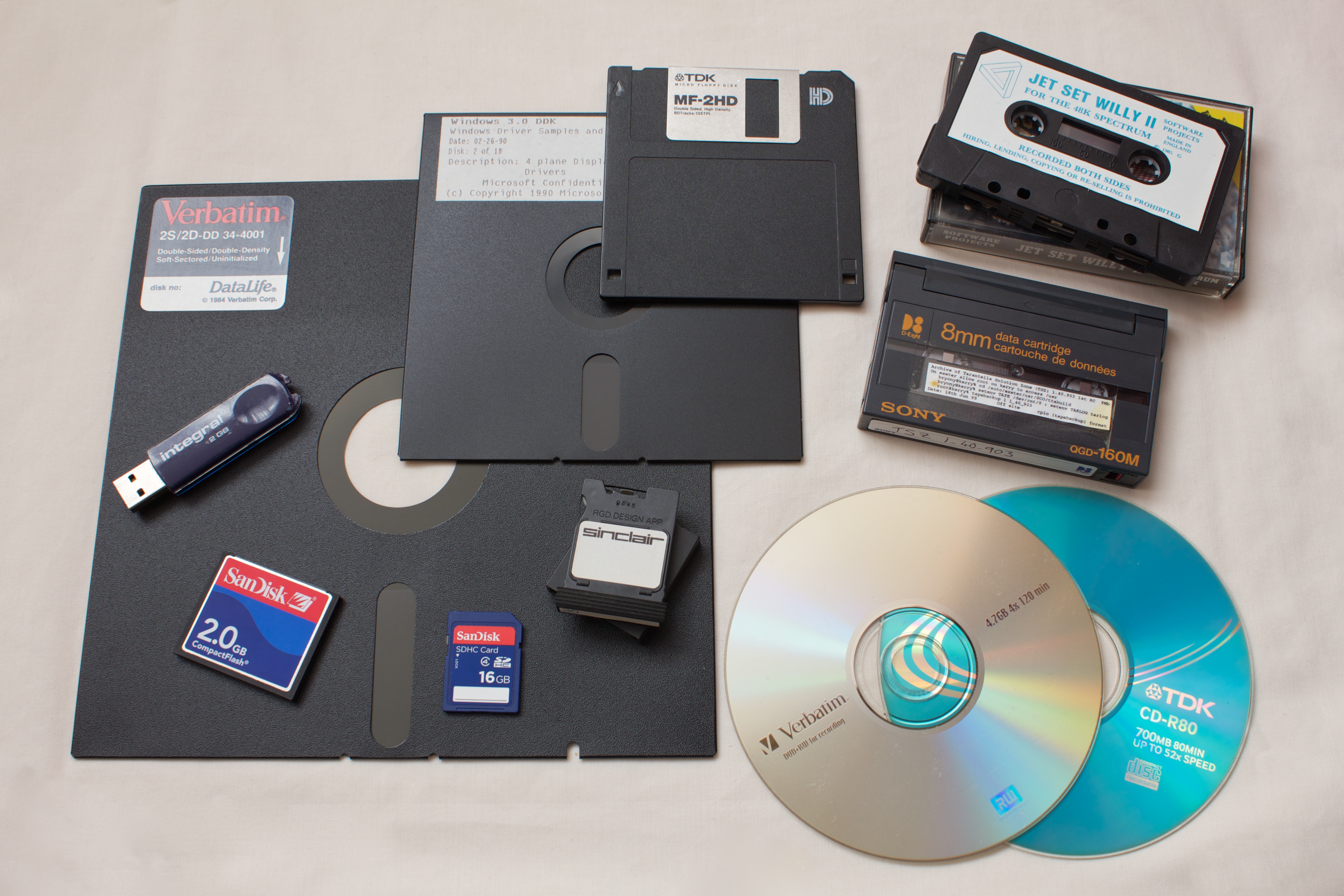
There are many types of permanent storage, but the most common type uses a “disk”, sometimes called a drive. Disks can be removed, but all computers have at least one internal disk which cannot be removed. Several types of removable disk are shown in Figure 6.2.

Data is stored on such a disk as follows:

1. Data on a computer is internally represented in binary numbers (1’s and 0’s).
   • Computers use binary numbers because it is easy to signify 2 values using high/low voltage, high/low resistance, high/low magnetism, etc.
2. Writing binary values to a disk is then done by applying some high/low signal to the disk.
   • For example, in the case of magnetic storage the values are created using a magnetic field to impart magnetism to the disk.
     
   • In the case of a CD, DVD, or BlueRay disk, the values are holes in a metal film on surface. In all cases, the disk holds these values as long as it’s not damaged or decayed by time.
3. Reading values from a disk is done by scanning over the disk surface and detecting the high/low values which were created during the writing process.
   • In the case of a magnetized disk the needle is a magnet that is attracted or repelled by the magnetic value on the disk.
     
   • In the case of a CD/DVD/BlueRay, a laser scans the disk and detects the reflection or lack thereof due to the holes.

By understanding a little bit about the disk reading/writing process, we can appreciate that it is a physical activity that requires moving parts and mechanical processes. Knowing this, we should not be surprized that reading and writing to a disk is a slow process. Therefore, if we are trying to write a fast program, we should avoid reading/writing to disk when possible.

Github Arctic Code Vault

Github has taken long-term storage to a new level.

Figure 6.2: The “save” icon in many programs is a picture of a removable floppy disk (shown in the upper-middle of the figure on the right), which is about as relevant to modern computers as an hour glass is to symbolize waiting.

6.1.2 Temporary Memory

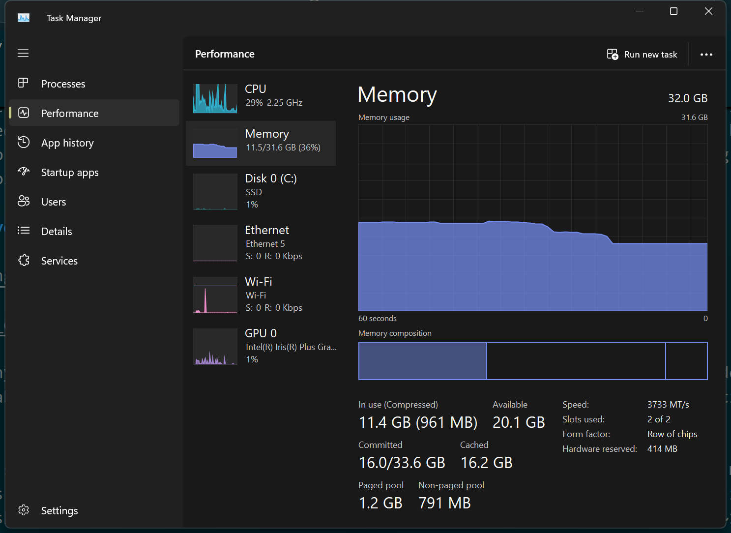
Computers also have a second type of memory, usually called RAM (Random Access Memory). RAM is much like ‘short term’ memory in humans. It is where we keep information which we are actively working on. RAM is designed to be much faster than a disk, but normally there is much less of it. A typical computer might have ~10 GB of RAM, while having ~1000 GB of disk space.

We typically use RAM as follows:

1. When we open a file, the PC retrieves it from the disk which can take an annoyingly long time
2. The data from the file is then loaded into RAM where we can read and write to it as needed.
3. Once we are finished with the file, we save it and close it. The computer then writes the updated data to the disk and purges the data from the RAM.

The RAM can become overfilled if we open too many large files. In this case the operating system will begin writing data to the disk. If you computer ever becomes noticeable and frustratingly slow, it is probably because this is happening.

Active memory vs long-term storage

The sum it all up, think of a information stored on disk as long-term, semi-permanent storage; while anything that the computer is currently working with is moved into active memory.

Figure 6.3: A screenshot of the Windows Task Manager showing RAM usage vs time. The dip occurred after closing all instances of my web-browser.

6.2 Files and Folders

When reading and writing data to the disk, the computer’s “operating system” (i.e. Windows, Mac, Ubuntu, etc.) presents us with a very familiar interface for dealing with stored data: files and folders.

Hidden file extensions

One extremely frustrating feature of Windows is that the file extension is hidden by default, so the files appear as “my_resume” instead of “my_resume.docx”. Enabling this visibility is a very good idea. This tutorial shows the process for several different versions Windows.

• Data is stored in files.
  • Common examples are are Word documents and images. We might have a Word document on our computer like my_resume.docx, or a picture like friends_at_pub.png.
  • The part after the last dot (.) is called the file extension.
  • The only purpose of file extensions is so the computer (and the user) know what program to use to open a file. If the extension was removed, you could still open it if you used the correct program.
  • For example, Outlook will not let you send a .py file because it could contain malecious code which the recipient might run. However, you can send code.py.temp or code.txt and Outlook will let it through. Then the recipient can change the extension back to .py.
• Files are stored in folders.
  • Common examples are your “downloads” or “documents” folder.
  • Folders can contain many files
  • Like real folders, folders can be stored inside other folders like /pictures/2020/January/PartyInNYC.
• Finally, folders are stored on a disk.
  • This is where the analogy to real world file systems breaks down because disks should be called “cabinets”.
  • A disk is a physical device inside the computer where data can be written. This is usually described as “storage”.
  • On Windows every disk is given a letter, with C:\ usually being the “main” drive.
  • On Mac the disk are not given letters, and they kinda all act like they are a folder themselves
• If we combine all of these together we get a path.
  • On Windows the path looks like:

C:\users\jeff\photos\ufo_sightings\591.jpg

• And on Mac it looks like:

/Home/jeff/photos/bigfoot_sightings/431.jpg

The above paths are considered absolute paths since they contain the entire path, from the disk letter all the way to the file. It is also possible to have relative paths which contain the part of the path below the currect directory. For instance, if we are currently in C:\users\jeff, then photos\ufo_sightings\591.jpg is a relative path to the file.

Note that Windows and Mac use different direction slashes. Recall the discussion about the use of escape characters when backslashes needed to be written (\\). This is particularly annoying on Windows since \ is used in the paths, while on Mac the / can be used without any escaping.

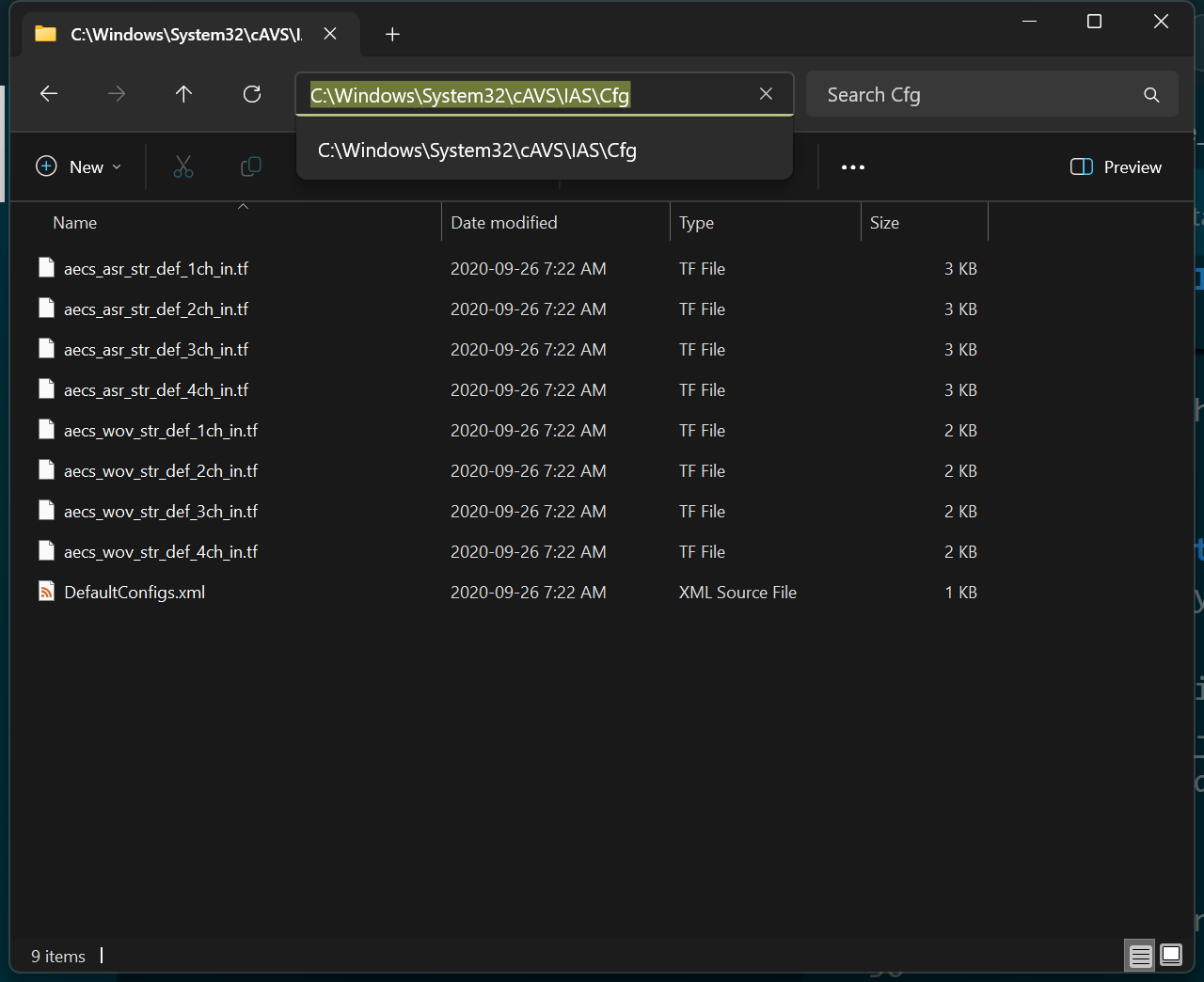
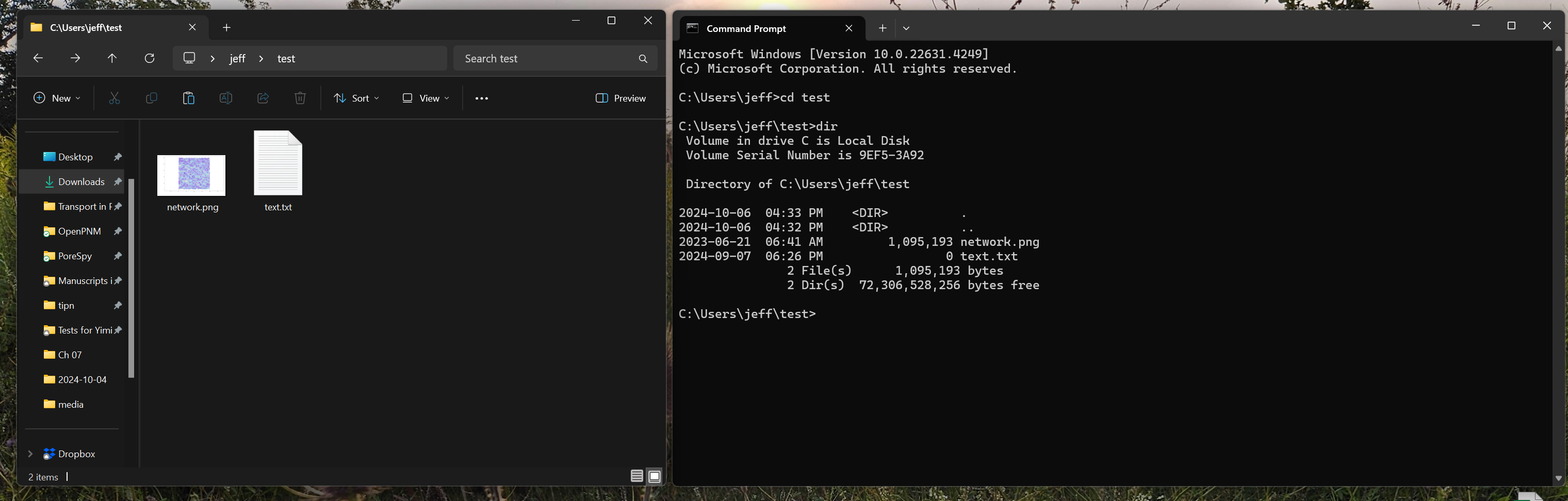
Below is a screenshot of a random folder deep within the Windows directory. Also shown is how title bar reports the absolute file path if you click it.

Figure 6.4: A screenshot of a file folder several levels deep into Windows

The point of storing files inside a hierarchical folder structure is for organization. Consider the file storage room in shown in Figure 6.5. If you are given a location (i.e. a path) in the form of aisle 8, section 4, shelf 4, box 11, page 10, line 55 you could find the exact sentence in a text file! The file system on a computer works exactly like this.

Figure 6.5: We could find a single sheet of paper in this pile, if given the right directions

6.2.1 Finder/Explorer vs Command Line

Now that we understand how our computer stores our files, we can appreciate what is happening when we browse our files using the Explorer in Windows (or Finder on Mac).

However, there is an alternative way to navigate our files: using the command line. Consider the following comparison:

Figure 6.6: Comparison of the graphical explorer view (left) and the command line approach to navigating the file system.

A major milestone on the path to becoming a proficient programmer is learning to use the command prompt (sometimes known as the command line or terminal). Modern operating systems provide gorgeous and powerful graphical user interfaces (GUIs), but ultimately our button clicks and checkboxes get translated into commands to be run by the computer. The command prompt lets us call such commands directly, bypassing the GUI. There are 2 main scenarios where we may need to do this:

1. As “power-users”, we often need to interact with the computer more directly than the GUI allows. The GUI hides many features and options since the vast majority of computer users do not need them.
2. There are many essential utility applications which do not have a GUI so must be activated from the command prompt.

The following table illustrates an example of working from the command prompt to open a text editor, in both Windows and Mac.

Table 6.1: A simple example of opening a text editor from the command prompts in Windows and Mac.

Windows	Mac
Press Windows key to open Start Menu	Type cmd+space to open Finder
Type cmd and press enter	Type terminal and press enter
At the “prompt” (C:\) type notepad	At the “prompt” type open -a TextEdit
When you press enter, the NotePad application will open up	When you press enter, the TextEdit app should open up
This is exactly equivalent to opening the start menu, typing “notepad” and clicking on the icon that appears.	This is exactly equivalent to opening Finder, typing “TextEdit” and pressing enter.

The number of commands that are available is enormous, and each one has different options. The following links provide “cheat sheets” for the most common and useful ones, to give a flavor of what is possible:

• A cheatsheet for Mac users is available here
• A cheatsheet for Windows users is available here

There are a few commands that are so common and useful that they are worth highlighting:

Listing contents of current directory	In Windows the command is dir, while in Mac it is ls.
Changing current directory	It is cd is both Windows and Mac. cd.. moves up one level, cd <folder> moves down to specified folder.

Example 6.1 (Navigating through the file system from the command line) Open the command propmpt on your computer and navigate to your “downloads” folder.

Solution

On Windows you can press the “Windows” key to get the menu, then type “cmd” or maybe “cmd.exe”, the click the result of the search (or press enter).

On Mac you can click the “Launchpad” icon, then type “terminal”, then click or press enter.

Once the terminal is open you can navigate using the following commands:

• cd .. moves up one level, cd\ moves to the top level
• dir/ls will list all files and folders in current directory
• cd <path> will move into the specified folder. Note that you can start typing <something>, then press the tab key to get an autocomplete.

Comments

Knowing how to use the command line, even just a little, is mandatory for an aspiring programmer.

6.3 Reading and Writing Text to a File

Figure 6.7: Most people have pretty bad file system hygiene.

6.3.1 Writing to a File

Writing text to a file is one of they ways we can make our data “permanent”, otherwise all of our calculations are lost when we shutdown our computers.

Because this is such an important task, Python has a built-in function for working with a file: open(). The open() command does not “open” a file physically for us to look at, they way Word does when we double-click a file name. Instead Python “opens” the door to the file so that data can flow in and out.

The general syntax is as follows:

1fname = 'data.txt'
2f = open(file=fname, mode='w')
3f.write('Hello world')
4f.close()

1

We define a str which we will use as our file name. The extension (the part after the .) is optional. Its only purpose is so that Windows/Mac knows which program to open the file with when you double-click it.

2

We use the open() function by passing in the name of the file and the ‘mode’ we wish to use. In this case the mode is 'w' which stands for “write”. The open() function returns a “file handle” which we store in f.

3

We can access a variety of methods attached to the file. The full list of methods is given in Table E.1, but a partial list is given below. In this case we use write() to write the given text.

4

It is necessary to close a file when done, otherwise it cannot be opened by other programs. Files generally need to be “locked” when in use so that multiple programs can’t write to it at the same time.

Where is my file?

If you create a file solely using a file name (i.e. no directory information), then the file will be created in Python’s “current working directory”. Luckily this is pretty easy to find:

1import os
2print(os.getcwd())

1

The os module has lots of functions for navigating your file system, as well as general information like the number of cores available, etc.

2

Here cwd stands for “current working directory”

This will return something like C:\Users\jeff\projects. If you navigate to this directory in your explorer/finder you will see your file (i.e. 'data.txt')

The result of writing “Hello world” to this file is shown in Figure 6.8 on the left:

Figure 6.8: The contents of the file after writing “Hello world”

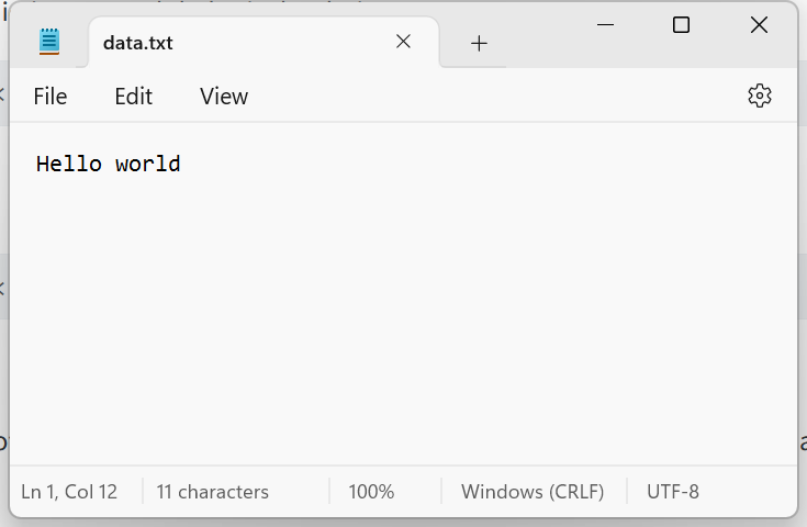
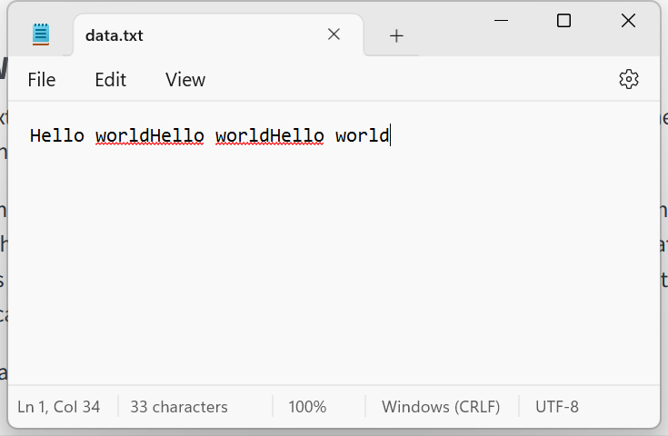
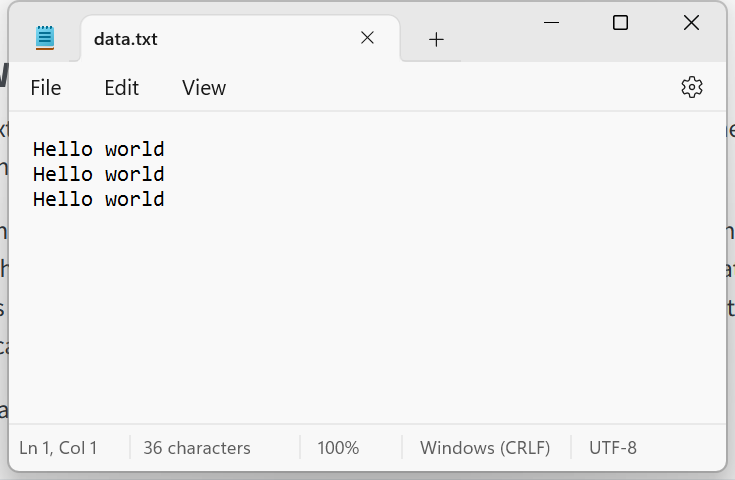
If we write to the file 3 times it will append the text to the existing text, creating one long line as shown in Figure 6.8 (middle)

fname = 'data.txt'
f = open(file=fname, mode='w')
f.write('Hello world')
f.write('Hello world')
f.write('Hello world')
f.close()

And finally, using our knowledge of escape characters we can add a new line after each write to get the result in Figure 6.8 (right)

fname = 'data.txt'
f = open(file=fname, mode='w')
f.write('Hello world\n')
f.write('Hello world\n')
f.write('Hello world\n')
f.close()

Example 6.2 (Write several lines of formatted text to a file) Write the current time and a random number to a file once per second for 5 seconds.

Solution

To solve this problem we will use 2 modules from Python’s standard library. To get the current time we will use time:

import time
print(time.ctime())

Sat Dec  7 15:05:30 2024

The ctime function converts the result of localtime to a human-readable string. localtime by contrast returns tuple with each component of the time in a different location like time.struct_time(tm_year=2024, tm_mon=9, tm_mday=2, tm_hour=11, tm_min=57, tm_sec=1, tm_wday=0, tm_yday=246, tm_isdst=1).

The time module also has a function called sleep which we will use to control the timing of the program.

The time module also contains a function called time() which returns the total number of seconds which have elapsed since “January 1, 1970”.

The random module contains functions for generating random numbers. (I wanted to use “real” data based on the temperature of your computer, but that requires installing external libraries).

1import time, random

2f = open(file='data.csv', mode='w')
3init_time = time.time()
4while (time.time() - init_time) < 5:
5    date_and_time = time.ctime()
6    value = random.randint(0, 1000)
7    s = date_and_time + ', ' + str(value) + '\n'
8    f.write(s)
9    time.sleep(1)
10f.close()

1

We import both time and random modules on the same line

2

We will write the data to a '.csv' file, which stands for “comma separated values”. Excel can/will open '.csv' file automatically.

3

We need to initialize the current time, which we will use determine when 5 seconds have elapsed.

4

Here we compute the difference between the current time and the time the program started. As long as this is less than 5 seconds, the while-loop will keep running

5

We use the ctime() function to get a text representation of the current time and date.

6

We generate a numerical value using the randint function. Here we have requested a number between 0 and 1000.

7

Here we format our text by adding a comma between the time and the value, convert the value to a string, and add a new line character at the end.

8

We write the formatted string to our file.

9

Since we only want to write data once per second we literally tell Python to take a nap for 1 second.

10

As always we have to close the file when we’re done.

Comments

We can open this file in Excel. Excel should automatically open when you double-click a '.csv' file. Try it and inspect the result. Remember to use os.getcwd() if you can’t find your file.

How to do X?

Here is a good time to reveal how I know about all these hidden features buried under so many levels of abstraction:

I Google it!

I use a search like “how to find the current time in python using standard library”. I usually look for the StackOverFlow links. Here is the page on StackOverflow. There are many answers, each proposing a different way to do it, complete with commentary by other coders and an upvote/downvote count to indicate how valuable the other users (like us!) found the answer.

6.3.2 Reading From a File

Reading data from a file not only let’s us reload data we may have written to a file, but it is also common to store tabulated data like constants and fitting parameters in files.

Let’s start with something simple to see how it works:

1f = open('file.txt', mode='w')
f.write('Hello world')
f.close()
2f = open('file.txt', mode='r')
3contents = f.read()
print("Result:", contents)

1

First we will open a new file and write “Hello world” in it so ensure there is file present.

2

Here we open the file in “read” mode ('r').

3

The read() function reads the entire contents of the file in to contents which we then print to see it contains 'Hello world'

Result: Hello world

Example 6.3 (Read complicated data from a file) Consider Antoine’s equation for predicting vapor pressure of a pure liquid as a function of temperature:

\[ log_{10}(P) = A - \frac{B}{T + C} \] where \(P\) is in units of \(mmHg\) and \(T\) is in units of \(^oC\). The values of \(A\), \(B\) and \(C\) are experimentally determined for each liquid, and their values are tabulated in various places. The data in Table 6.2 are an example from a file that was over 14 pages long.

Table 6.2: Antoine coefficient data for 13 species taken from a list over 14 pages long

ID	Formula	Compound Name	A	B	C	Tmin	Tmax
1	CCL4	carbon-tetrachloride	6.89410	1219.580	227.170	-20	101
2	CCL3F	trichlorofluoromethane	6.88430	1043.010	236.860	-33	27
3	CCL2F2	dichlorodifluoromethane	6.68619	782.072	235.377	-119	-30
4	CCLF3	chlorotrifluoromethane	6.35109	522.061	231.677	-150	-81
5	CF4	carbon-tetrafluoride	6.97230	540.500	260.100	-180	-125
6	CO	carbon-monoxide	6.24020	230.270	260.010	-210	-165

Let’s explore the process of reading this kind of data in from a file. We will load the data into dicts so that we can access it using the very convenient syntax of data['CCL4']['A'].

Solution

The first thing we need to do is create a file with formatted data. This way the file will exist in our current working directory and we can avoid the complication of searching for it (we’ll deal with that later).

So, let’s format the data as ‘comma separated values’:

1data = [
2    "ID, Formula, Compound Name, A, B, C, Tmin, Tmax\n",
3    "1, CCL4, carbon-tetrachloride, 6.89410, 1219.580, 227.170,-20, 101\n",
    "2, CCL3F, trichlorofluoromethane, 6.88430, 1043.010, 236.860, -33, 27\n",
    "3, CCL2F2, dichlorodifluoromethane, 6.68619, 782.072, 235.377, -119, -30\n",
    "4, CCLF3, chlorotrifluoromethane, 6.35109, 522.061, 231.677, -150, -81\n",
    "5, CF4, carbon-tetrafluoride, 6.97230, 540.500, 260.100, -180, -125\n",
    "6, CO, carbon-monoxide, 6.24020, 230.270, 260.010, -210, -165\n",
]

4f = open('coefficients.csv', 'w')
5f.writelines(data)
f.close()

1

We are putting each line as a str inside a list. This is a classic use of collections to hold many pieces of data at once.

2

This line is called the header. We will have to remember to remove this when we read the data back

3

Each line from the table is written as it’s own string, ending with a '\n'.

4

We open a new file in ‘write’ mode.

5

Here we are using a new function writelines() which write each str in a list to the file. We could have used a for-loop and called write() for each item in data.

Now we are ready to read this data in from the file we just created:

f = open('coefficients.csv')
1header = f.readline()
2database = dict()
while True:
3    txt = f.readline()
4    if txt == '':
5        break
6    txt = txt.split(', ')
    coeffs = {}
7    coeffs['A'] = txt[3]
    coeffs['B'] = txt[4]
    coeffs['C'] = txt[5]
    chem_name = txt[1]  
8    database[chem_name] = coeffs

1

Read the first line to get past the header

2

Create an empty dict to hold the incoming data

3

Read a single line into txt

4

If the value of txt is '' is means we have reached the end of the file

5

The break() command will immediately end any for or while loop that is running

6

We use the split() function to break the string at each occurrence of , and put each piece into a list. Each list entry will therefore correspond to a column in the file.

7

We need to have some knowledge of how the data is organized in the file. Here use the fact that the coefficients are stored in columns 3, 4 and 5, and the chemical formula is stored in column 1.

8

We finally assign coeffs to the database under the chemical formula.

Now we can use our database as follows:

A = database['CCL4']['A']
B = database['CCL4']['B']
C = database['CCL4']['C']

We have done something a bit fancy here: we used nested dictionaries. The database variable is a dict, but the item stored in each element is also a dict. If this makes your brain hurt, we can do an equivalent look-up as follows:

coeffs = database['CCL4']
A = coeffs['A']
B = coeffs['B']
C = coeffs['C']

Comments

This example showed us quite a few new tricks in Python:

• Nested dictionaries
• break statements
• String splitting
• And of course reading from a rather complicated file

6.4 Installing External Packages

We have already seen that Python includes many additional packages as part of the “standard library”. These provide functionality that is often important, but not necessary for everyone. The programmer can therefore import the extra functionality when needed.

Although Python’s standard library is considered very good (compared to most languages), it cannot possibly consider everything. For this reason we can install “external packages” from a variety of sources. The most common source is The Python Package Index or PyPI.

Installing packages happens to be one of the reasons why a competent programmer should be comfortable using the command line. We usually install packages by opening the operating system’s command prompt and typing pip install <package-name>. However, it is not quite that simple because it depends on how Python was installed.

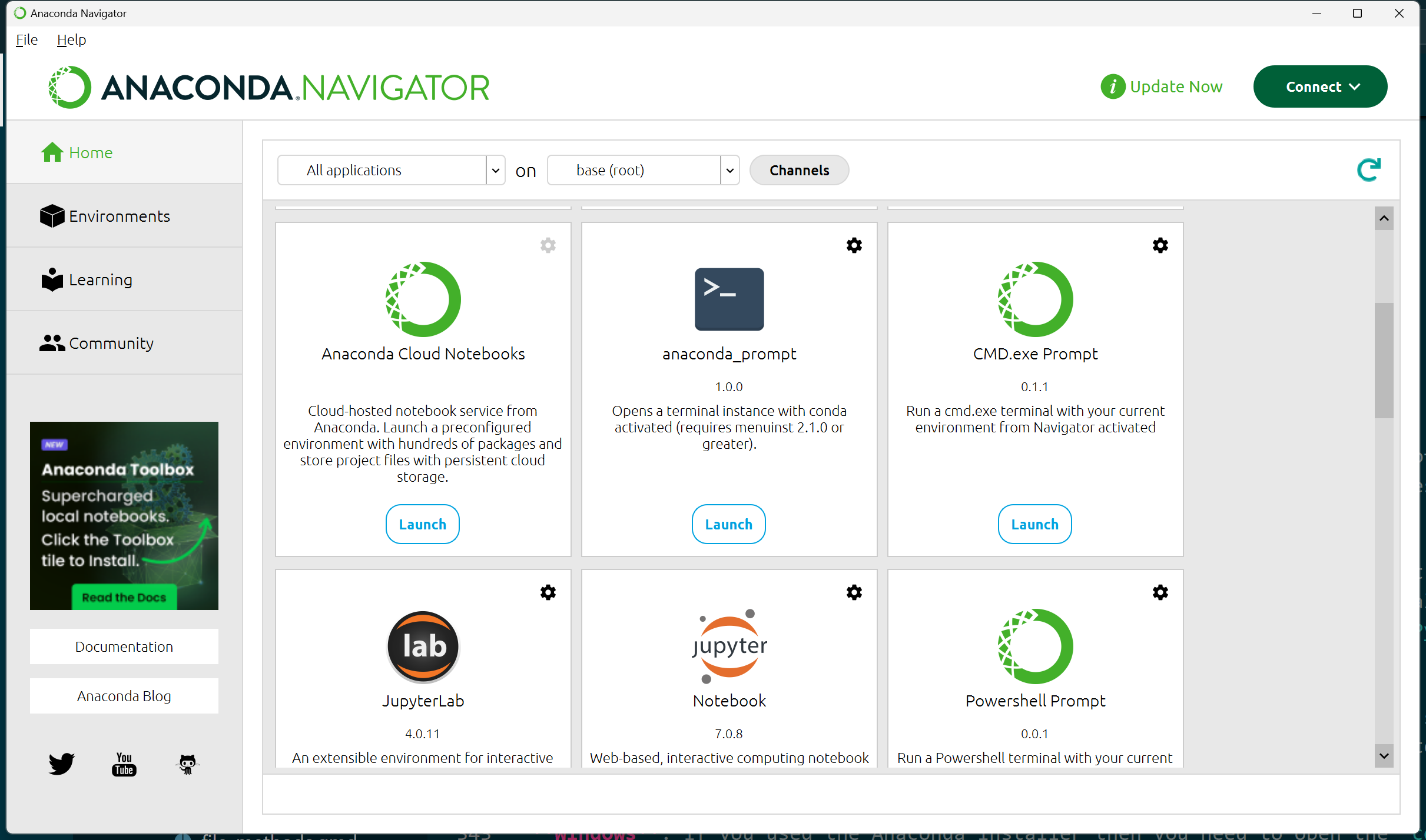
It is possible to install packages using the Anaconda Navigator interface. However, for reasons that are difficult to explain, this fetches packages from somewhere other than PyPI, so offers an incomplete selection.

For our purposes, we can avoid complications by using the anaconda_prompt via the Anaconda Navigator.

The Anaconda Navigator

The Conda Prompt

Figure 6.9: The (Ana)Conda Prompt can be accessed via the Anaconda Navigator user interface.

pip is sometimes slow

Because the installation of external packages is very central to using Python, there are several other tools which have been built to provide the same functionality. Very recently a packages called uv was released with works amazingly well. To use it, you first need to install it with pip install uv, since it installs just like a normal Python package.

Once you have uv installed, you can use it with uv pip install <package>. The pip “subcommand” provides a nearly drop-in replace for real pip, but is about 100x faster. uv has lot of other features too, but we’re not ready to appreciate them yet.

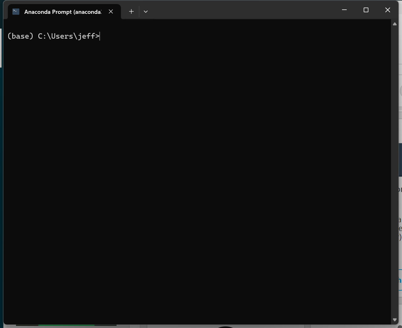
This “prompt” has special capabilities, including the ability to use pip without any additional setup. Test that pip is available and working by typing:

(base) C:\> pip list

This will give you a list of all packages that are currently installed. What this line does is the following:

1. Runs a program on your computer called pip
2. Every other item on the line gets passed to pip as an argument, in much the same way arguments are passed to functions.
   
3. pip will run using the arguments you passed, and do something. In this case is prints a list of all installed packages.

Example 6.4 (Install a package using pip) pandas is known as “Excel for Python”. It let’s us perform operations on tabular data. Probably the most common use of pandas is to read and write csv files.

Download the csv file found here and open it using pandas.

Solution

Clicking the above link will probably result in the file being downloaded to your computer, and placed in the downloads folder.

In Spyder, we will create the following script:

import pandas as pd

p = <path to file>  # Here we will put the actual path!
data  = pd.read_csv(p)

This probably did not work. pandas will be installed on your system (it’s included with Anaconda), but openpyxl is not installed by default. pandas will try to use this package and tell you that it cannot be found. So let’s install it.

1. Open the “conda prompt”.
   
2. Type pip install openpyxl
3. Wait while pip downloads the requested package and all the dependencies.
4. Try script again.

This time pandas should have succeeded.

The data variable will be specialized dict, which has all the usual dict methods plus a LOT more.

Try:

print(data.keys())

Which should give:

Index(['ID', 'Formula', 'Compound', 'A', 'B', 'C', 'Tmin', 'Tmax'], dtype='object')

Now let’s fetch values using some of pandas special features. We already know how to get a full column from a dict (i.e. data[key]), but pandas let’s us get a full row using the loc method:

vals = df.loc[df['Compound'] == 'cyclohexane']

vals looks like this:

      ID Formula     Compound       A         B        C  Tmin   Tmax
268  269   C6H12  cyclohexane  6.8413  1201.531  222.647     6  105.0

Comments

In this example we have used an external package (pandas) which itself used another external package (openpyxl) which we installed ourselves. This is a very common situation when using Python.

Now that we have the ability to to install and use more complicated packages, we can revisit some tasks and do them differently.

Example 6.5 (Repeat Example 6.2 using pandas) Instead of writing data directly to a file line-by-line, collect the data in a dict, then write the entire dataset to a csv file using pandas.

Solution

import time, random
1import pandas as pd

2data = {'date_and_time': [], 'value': []}
init_time = time.time()
while (time.time() - init_time) < 5:
    data['date_and_time'].append(time.ctime())
    data['value'].append(random.randint(0, 1000))
    time.sleep(1)

3df = pd.DataFrame(data)
4df.to_csv('data2.csv')

1

Import pandas at the top since we know we’ll be using it

2

Initialize a dictionary with the desired keys, and set values to empty list which we will append data to on each loop.

3

Excel calls them ‘sheets’, pandas calls them ‘DataFrames’. Here we initialize a new DataFrame, and populate it with data. pandas will use the keys as column headers, and fill each column with the corresonding values.

4

Just as pandas offers a read_csv method, it also offers a to_csv method.

The output would look like this:

	date_and_time	value
0	Sun Oct 6 19:46:58 2024	624
1	Sun Oct 6 19:46:59 2024	671
2	Sun Oct 6 19:47:00 2024	681
3	Sun Oct 6 19:47:01 2024	407
4	Sun Oct 6 19:47:02 2024	175

Comments

The overall message here is not “use pandas”, but more generally “there is probably a package that already does some tedious work that I can use instead of coding it up by hand”.

6.5 Excercises

Instead of exercises, just work directly on Assignment 4.