9 Numerical Computing Part 2: Using Numpy and Scipy

Last lecture we learned about Numpy and how it solves the problem of slow for-loops: It basically provides hundreds of pre-written functions to do the common things for which we’d normally need to write a for-loop.

Numpy saves us coding time as well

These functions are both much faster than what we could write in Python, but they also save us time since we don’t have to write code for a bunch of common operations. So even if Numpy was not built on highly efficient C-based code, we’d still use it (or something like it) to perform all the routine functions for numerical arrays.

In this chapter we’ll learn about a few more techniques that Numpy offers to help us avoid writing complex code ourselves. Among other things, we’ll start learning about using Numpy for linear algebra and other mathematical operations.

Figure 9.1: Numpy provides us with access to some of the worlds most rigorous and established code for mathematical computations. In this case BLAS stands for “Basic Linear Algebra Subroutines”.

9.1 Broadcasting

Last lecture we learned about “element-wise” operations, where we could do an operation between a scalar and an array:

import numpy as np

arr = np.array([1, 2, 3])
arr2 = arr + 10.0
print("The result of adding a scalar to an array is:", arr2)

The result of adding a scalar to an array is: [11. 12. 13.]

Or operate two arrays of the same size:

arr1 = np.array([1, 2, 3])
arr2 = np.array([11, 12, 13])
arr3 = arr1 + arr2
print("The result of adding two arrays (of matching shape) is:", arr3)

The result of adding two arrays (of matching shape) is: [12 14 16]

But Numpy also let’s us do operations on arrays with different shape…as long as the shapes are compatible. This is called broadcasting and it works as follows:

1arr1 = np.ones((2, 3))*100
print(arr1)

2arr2 = np.arange(3)
print(arr2)

3arr3 = arr1 + arr2
print(arr3)

1: Create an array of shape (2, 3)
2: Create an array of shape (3,)
3: When we add them we see that arr1 gets added to each row of arr2

[[100. 100. 100.]
 [100. 100. 100.]]
[0 1 2]
[[100. 101. 102.]
 [100. 101. 102.]]

There are actually three scenarios where broadcasting is invoked:

Rules of Broadcasting

Rule 0: If using a scalar and an array of any shape, the scalar will be applied to every element in the ndarray. This one is not an official rule, but is worth including this list to remind us that operations using scalars are a form of broadcasting.
Rule 1: If the two arrays differ in their number of dimensions, the shape of the one with fewer dimensions is padded with ones on its leading (left) side.
Rule 2: If the shape of the two arrays does not match in any dimension, the array with shape equal to 1 is stretched in that dimension to match the other shape.
Rule 3: If in any dimension the sizes disagree and neither is equal to 1, an error occurs.

Figure 9.2 shows a few examples of broadcasting arrays of different shapes:

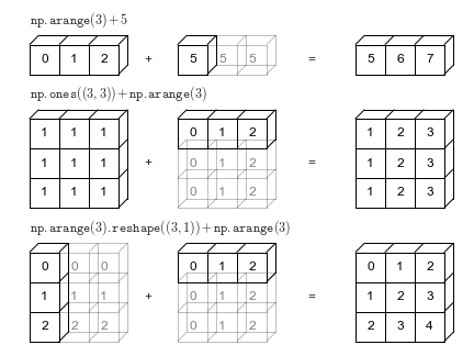
Figure 9.2: The act of “broadcasting” arrays of different shapes. The top row shows the case when a scalar is added to a 1D array, or Rule 0. The middle row shows an example of Rule 1. The bottom row shows an example of Rule 2.

Let’s see each of these in action.

9.1.1 Broadcasting: Rule 1

We have already seen this one, but let’s look again. If we have a 2D array and a 1D array, we can multiply them together, and the result will be a 2D array:

arr2d = np.ones((3, 4))*10
arr1d = np.arange(4)
arr = arr1d*arr2d
print(arr)

[[ 0. 10. 20. 30.]
 [ 0. 10. 20. 30.]
 [ 0. 10. 20. 30.]]

In this case Numpy takes arr1d and adds a new dimension at the beginning of the list of dimensions, then duplicates the values from the original dimension. This is like using vstack on arr1d 3 times. In fact we can recreate this behavior ourselves:

arr2d = np.ones((3, 4))*10
arr1d = np.arange(4)
1arr1d_stacked = np.vstack((arr1d, arr1d, arr1d))
arr = arr1d_stacked*arr2d
print(arr)

1: Here we manually counted how many times we need to stack arr1d and “hard-coded” this value when we called vstack().

[[ 0. 10. 20. 30.]
 [ 0. 10. 20. 30.]
 [ 0. 10. 20. 30.]]

“Hard-coding” values like this is bad practice, since it will obviously only work for arrays of that specific shape. We can do this is a more abstract way using the tile function as follows:

arr2d = np.ones((3, 4))*10
arr1d = np.arange(4)
1arr1d_tiled = np.tile(arr1d, [arr2d.shape[0], 1])
arr = arr1d_tiled*arr2d
print(arr)

1: Here we tell Numpy to tile the input array (arr1d) N times, where N is take from the shape of arr2d. This way the code it totally general for any shape of arr2d.

[[ 0. 10. 20. 30.]
 [ 0. 10. 20. 30.]
 [ 0. 10. 20. 30.]]

For the sake of completeness, we could also use some of the built-in Python features to broadcast the lower-dimensional array ourselves:

arr2d = np.ones((3, 4))*10
arr1d = np.arange(4)
arr1d_pythonic = np.array([arr1d]*arr2d.shape[0]).reshape(arr2d.shape)
arr = arr1d_pythonic*arr2d
print(arr)

[[ 0. 10. 20. 30.]
 [ 0. 10. 20. 30.]
 [ 0. 10. 20. 30.]]

9.1.2 Broadcasting: Rule 2

If both arrays are 2D but not the same shape, Numpy will duplicate the “lower dimensional” array along its “singleton” axis, assuming it has one.

Singleton axis

When an array has a singleton axis it means that the shape in that dimension/axis is 1. Sometimes singleton axes are necessary so that arrays can be compatible with each other. Other times the singleton axis is redundant and can be removed.

arr = np.ones((1, 3, 3))
print(arr)

[[[1. 1. 1.]
  [1. 1. 1.]
  [1. 1. 1.]]]

Note that this array is nested inside three sets of [ ], indicating a 3D array.

We can use the np.squeeze() function to removes singleton dimension(s):

arr = np.ones((1, 3, 3))
arr = np.squeeze(arr)
print(arr)

[[1. 1. 1.]
 [1. 1. 1.]
 [1. 1. 1.]]

Note that missing set of [ ] around this array, indicating it’s been reduced to 2D.

arr2d = np.ones((3, 3))*10
arr2d_singleton = np.arange(3).reshape((3, 1))
arr = arr2d*arr2d_singleton
print(arr)

[[ 0.  0.  0.]
 [10. 10. 10.]
 [20. 20. 20.]]

When operating on a pair of arrays with the same dimensionality, Numpy doesn’t care which dimension it needs to tile along, so broadcasting will also work in this case:

arr2d = np.ones((3, 3))*10
arr2d_singleton = np.arange(3).reshape((1, 3))
arr = arr2d*arr2d_singleton
print(arr)

[[ 0. 10. 20.]
 [ 0. 10. 20.]
 [ 0. 10. 20.]]

9.1.3 Broadcasting: Rule 3

The final broadcasting rule basically states that if Rules 1 or 2 don’t work, then an error occurs.

The obvious case is when the dimensions are fundamentally incompatible in both directions:

arr1 = np.ones((3, 3))*10
arr2 = np.arange(8).reshape((2, 4))
try:
    arr3 = arr1*arr2
1except ValueError as e:
    print(e)

1: Now that we know about try/except blocks, here is a useful case. You can catch the error then print it, instead of having it halt your code. Of course this is only a good idea for things like notes and tutorials. In reality you want your code to halt if there is a problem.

operands could not be broadcast together with shapes (3,3) (2,4)

There is just no way to that arr2 could be altered, rotated, or tiled to match the shape of arr1.

Rule 3 also applies even when one of the arrays does have a singleton dimension:

arr1 = np.ones((3, 3))*10
1arr2 = np.arange(4).reshape((1, 4))
try:
    arr3 = arr1*arr2
except ValueError as e:
    print(e)

1: arr2 has a size of 4 in the 2nd dimension, while arr1 has shape of 3 in both, so no broadcasting is possible.

operands could not be broadcast together with shapes (3,3) (1,4)

Consider the more subtle case where we have a common size in one dimension, but neither array has a singleton axis:

arr2d = np.ones((3, 3))*10
arr2d_no_singleton = np.arange(6).reshape((2, 3))
try:
    arr3 = arr2d*arr2d_no_singleton
except ValueError as e:
  print(e)

operands could not be broadcast together with shapes (3,3) (2,3)

It is important to understand why this case fails: It is because Numpy does not know what data to put in the new row. In the case of a singleton axis it is obvious that the values in that dimension should be copied, but in the case of a (2, 3) array, there is no clear choice for which data to put in row 3.

9.2 Ufuncs

So far we have seen that the Numpy library offers several functions at the “top-level” (i.e. np.<func>). We have focused on the “utility” functions, such as:

np.array() converts a list of values into an ndarray, which is Numpy’s special data-type.
Functions for merging, splitting and reshaping arrays, like np.vstack(), np.split(), and np.reshape()
Functions for generating new arrays like np.ones(), np.zeros(), and np.arange().

In addition to these utility-type functions, Numpy also offers a large variety of mathematical and numerical functions. These are officially called “ufuncs” for Universal Functions.

The list of available functions is too long to reproduce here, so the links below take you to the Numpy documentation:

9.2.1 Ufuncs that Operate on a Single Array

Some of the functions offered by Numpy perform an operation on a single array, such as the trigonometric functions like np.cos(), or the mathematical functions like np.log10().

These work on 1D arrays:

arr = np.arange(4)
res = np.cos(arr)
print(res)

[ 1.          0.54030231 -0.41614684 -0.9899925 ]

And ND arrays:

arr = np.arange(4).reshape((2, 2))
res = np.cos(arr)
print(res)

[[ 1.          0.54030231]
 [-0.41614684 -0.9899925 ]]

Warning

Even though the math library in Python’s standard library has a cos function, it does not work on ndarrays. If you attempt to do the following, you will get an error message:

from math import cos
arr = np.arange(4)
cos(arr)

Only the Numpy functions are able to operate on the Numpy arrays in the element-wise fashion that we want.

9.2.2 Ufuncs that Operate on Pairs of Arrays

Other functions operate on 2 arrays, such as add and multiply. These functions work exactly like the corresponding mathematical operator. For instance, addition using np.add() and using + are identical:

arr1 = np.ones((1, 3))*10
arr2 = np.ones((3, 3))
res = arr1 + arr2
print(res)

[[11. 11. 11.]
 [11. 11. 11.]
 [11. 11. 11.]]

and

arr1 = np.ones((1, 3))*10
arr2 = np.ones((3, 3))
res = np.add(arr1, arr2)
print(res)

[[11. 11. 11.]
 [11. 11. 11.]
 [11. 11. 11.]]

Combined functions

Some of the functions do multiple calculations in a single call. These are offered for convenience. For instance, np.logaddexp() is the same thing as calling np.log(np.exp(x1) + np.exp(x2)).

Example 9.1 (Compute the area under a curve) The graph below describes the power consumption of a house at hourly increments over the course of a day. Find the total amount of energy consumed and the corresponding electricity bill if it costs $0.18/kW-hr.

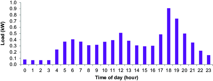
The data have been extracted from the graph and are given below:

t = [0,    1,    2,    3,    4,    5,    
     6,    7,    8,    9,    10,   11,   
     12,   13,   14,   15,   16,   17,   
     18,   19,   20,   21,   22,   23]
P = [0.08, 0.07, 0.07, 0.06, 0.23, 0.38, 
     0.40, 0.38, 0.33, 0.33, 0.37, 0.38, 
     0.51, 0.37, 0.32, 0.31, 0.32, 0.48, 
     0.92, 0.75, 0.51, 0.36, 0.22, 0.18]

Solution

Recall that power has units of $W = J/s$, while energy has units of $J$. When we consume $1J$ for $1s$, we use a $W$ of power.

The usage of electricity is charged based on the total amount of energy we consume. In other words if we slowly charge our phone by injecting $1 J$ each second for an hour we’ll use 3600 J, and if we rapidly charge it by injecting 3600 $J$ in a single second, we pay the same. (Note: because of inefficiencies in the way batteries work, doing it slowly will result in more charge in the battery, while doing it quickly will generate a lot of heat that is not useful, but this is another story).

As shown in the plot above we consume more power during some time periods and less in others. To find the total energy consumed we must find the area under the curve, which would give us units of $kW \cdot hours$.

There are a few ways we could tackle this. In the present case, the data points are equally spaced and on an hourly basis, so we could just note that each bar is essentially the energy used during each hour, then add up the y-values. But let’s make a more robust solution:

Let’s assume that the data points could be unequally spaced.
Let’s also assume a linear transition between hourly values. For example, instead of assuming that between 19:00 and 19:59 the power consumption was 0.75, lets assume that it starts 0.75 at 19:00 and decreases linearly to 0.51 by 20:00.

Firstly let’s convert our data to ndarrays:

t = np.array(t)
P = np.array(P)

Let’s plot the data in a few different formats:

import matplotlib.pyplot as plt

fig, ax = plt.subplots(figsize=[5, 5])
ax.step(t, P, where='post')
ax.plot(t, P, 'r.')
ax.plot(t, P, 'g-')
ax.set_ylim([0, 1])
ax.set_ylabel('Hourly power usage [kW]')
ax.set_xlabel('Time of day [hr]');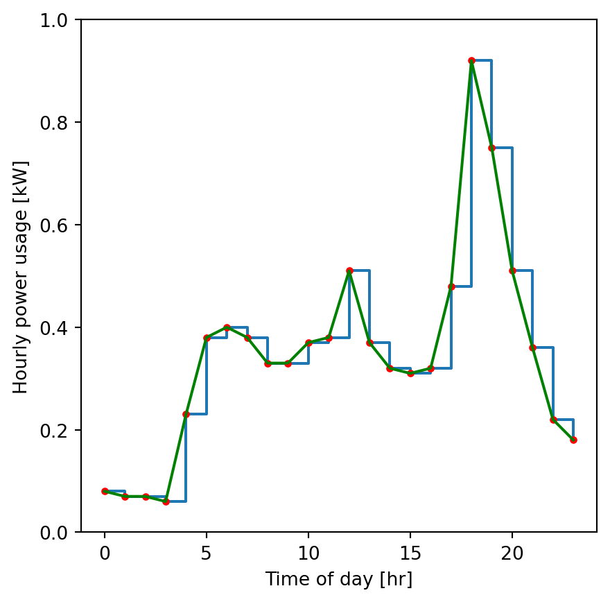

Now let’s integrate this data. We need to compute the area of the trapezoids defined by the green line above. The area of a trapezoid can be found from the area of a rectangle plus the area of the triangle sitting on top. However, an easier way it to use the average height of the left and right sides of the trapezoid.

This dataset presents a challenge that we must remedy first: There is one data point per hour for a total of 24 points, but we actually need 25 points. We need to connect the last data point at 11pm to the data point for 12AM the following day so that we can compute the average power usage from 11-11:59pm. Let’s assume the value from 12AM of the current day is a good estimate for the following day. We can update the data as follows using the reshaping/stacking routines:

P = np.hstack((P, P[0]))
t = np.hstack((t, [25]))

Now we can find the average power used during each hour. We’ll add the power values from t+1 to t, then divide by 2:

Pave = (P[1:] + P[:-1])/2

We also need to the spacing between data points, which might not be equal. Numpy has a function for this:

delta_t = np.diff(t, 1)

Now let’s find the area under the curve:

E = np.sum(Pave*delta_t)
print(E)

8.46

The total energy used during this day was 8.46 kW-hrs.

The cost of electricity is $0.18 per kW-hr, so the electricity bill for this day can be found as:

C = E*0.18
print("The daily electricity cost is: $", round(C, 3))

The daily electricity cost is: $ 1.523

Comments

This example shows off several of Numpy’s features:

Array initialization
Array reshaping
Slice notation
Use of Numpy’s built-in “Ufuncs”
Element-wise multiplication

In addition to “using” Numpy, we also add to “reason” about the mathematics of the problem:

Adjust the array size so we could incorporate the first value from the next day
Allow for unequal spacing in our time data
Improve the estimate of the power usage by averaging the values for each time period.

Basically, this example is a fairly good illustration of Numpy at work. Even though we were working with several lists of data, and needed to do a few fancy calculations, we still managed to avoid any for-loops.

9.3 Numpy’s Modules

Numpy includes several modules containing “application specific” functions that are common enough that they are included in Numpy, rather than a separate package. These including the following “numerical” features:

And the following “utilities”:

Let’s take a closer look as some of these.

9.3.1 The `numpy.random` Module

One of the main uses of this module is to generate random values from a specified distribution. These distributions will be more relevant once you’ve taken a course in statistics, but consider the following:

arr1 = np.random.rand(10000)
arr2 = np.random.normal(0.5, 0.1, 10000)

fig, ax = plt.subplots(figsize=[5, 5])
ax.hist(arr1, edgecolor='k', label='uniform', alpha=0.75)
ax.hist(arr2, edgecolor='k', label='normal', alpha=0.75)
ax.legend()
ax.set_xlabel('Value')
ax.set_ylabel('Number of occurrences in stated range');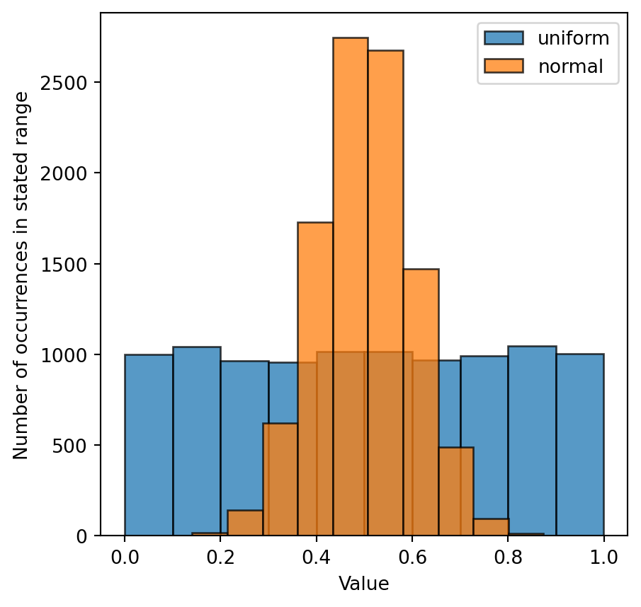

Figure 9.4: Comparing a normal and a uniform distribution of 10,000 points

An partial list of functions for generating data from different distributions is given below:

beta
binomial
exponential
gamma
logistic
lognormal
normal
pareto
poisson
power
rand
randint
rayleigh
vonmises
weibull

Each of these distributions is relevant to some different physical system. The normal distribution is good for describing things like height or weight of a group of people. The weibull distribution is useful for describing manufacturing and production rates. The functions in numpy.random are quite basic only useful for generating values. To do more detailed analysis of statistical data you can use scipy.stats.

9.3.2 The `numpy.linalg` Module

The linalg module contains all the functions you would expect for performing “matrix” operations, such as dot-products, cross-products, matrix multiplication, and finding eigenvalues.

9.3.2.1 `matmul`

Helper or Convenience Functions

Some of the functions in the linalg module are so commonly used that they are also included in the top-level namespace of the Numpy package for convenience. For instance, np.matmul just calls np.linalg.matmul, but it saves the programmer some typing.

Matrix multiplication is the most important computer operation in all of engineering and science. This is because the mathematical description of many physical systems yields a “system of coupled linear equations”. We must solve this system of equations to find the values of the physical process.

Fully appreciating this fact might require a few more years of coursework. But let’s take a quick look at a “resistor network” problem, which occurs in electric circuits, but is also used as an analogy for many other systems such as fluid flow in pipes.

Example 9.2 (Matrix multiplication with a system of equations) Consider a network of 6 resistors, arranged as shown in Figure 9.5. The resistors all have a random conductance, $G$, between 1 and 4, indicated by their color. (Note that conductance is the inverse of resistance, so $G=1/R$). Electrons preferentially follow the path of least resistance as they traverse the network, so the flow through each resistor will not be equal. As engineers analyzing this system, we would like to know things like (a) the voltage at each node, (b) the current in each resistor, and (c) the total total current flowing through the network.

The voltage in each node was measured as:

V = [2.0, 2.0, 1.51515152, 1.36363636, 1.0, 1.0]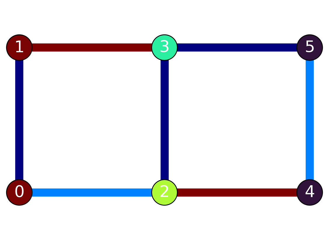

Solution

The current flowing in each resistor is given by Ohm’s law:

\[ I = G \cdot (V_j - V_i) \]

This tells us that if we know the voltage difference across a given resistor we can find the current, $I$, flowing through it.

Let’s assume that the voltage values in each node are known from some experimental measurements. How might we proceed to find the current flowing through the network? This is where matrix multiplication comes in.

First we need to set up a matrix containing the information about how current is exchanged between nodes. We can invoke the fact that current is conserved, so that current entering a node from all its neighbors is equal to the current that leaves. Referring to Figure 9.5, we can see that Node 0 is connected to nodes 1 and 2. A current balance around node 0 gives:

\[ G_{0,1} (V_1 - V_0) + G_{1,2} (V_2 - V_0) = 0 \]

This equation is written such that current flow from the neighboring nodes into node 0 is positive. If the voltages are reversed then the “inward” flow will be negative. This equation also states that the net flow will be 0, meaning that the inward flow is equal to the outward flow, and there is no accumulation in the node.

Now let’s rearrange this equation to “matrix” form by grouping coefficients accordingly to voltage value to which they are associated:

\[ -(G_{0,1} + G_{1,2})V_0 + (G_{0,1})V_1 + (G_{1,2})V_2 + 0V_3 + 0V_4 + 0V_5= 0 \]

The above equation represents the first row of a “coefficient matrix”, $A$. The 0’s mean that no current is exchanged between node 0 and 3, 4 or 5. Writing a balance equation for the other 5 nodes and inserting the numerical values for the conductances, yields the full matrix:

A = [[-5.,  3.,  2.,  0.,  0.,  0.],
     [ 3., -4.,  0.,  1.,  0.,  0.],
     [ 2.,  0., -6.,  3.,  1.,  0.],
     [ 0.,  1.,  3., -7.,  0.,  3.],
     [ 0.,  0.,  1.,  0., -3.,  2.],
     [ 0.,  0.,  0.,  3.,  2., -5.]]

To find the current flowing through each node we can now invoke Ohm’s law in matrix form:

\[ I = AV \]

Note that the $\DeltaV$ is replaced with just $V$ because the deltas are all now incorporated in the $A$ matrix.

We will use the voltage values that were measured in each node. Note that the form of this data is a vector like $(V_0, V_1, ..., V_n)$.

V = np.array(V)

Now, we can use np.linalg.matmul() to multiply the coefficient matrix by the voltage values. The result is the net current flowing through each node:

I = np.linalg.matmul(A, V)
print(I.reshape((I.size, 1)))

[[-9.69696960e-01]
 [-6.36363640e-01]
 [-4.00000006e-08]
 [ 3.99999998e-08]
 [ 5.15151520e-01]
 [ 1.09090908e+00]]

The results are returned as a “vector” of $I$ values of the same shape as the given $V$ values.

Comments

The solution tells us a few things:

The current flowing through the internal nodes $2$ and $3$ is indeed (nearly) $0$ as expected based on the assumptions used when writing the balance equations.
The nodes on the left ($0$ and $1$)and on the right ($4$ and $5$) have non-zero current. This is because these nodes are “boundary” nodes.
The negative current on the left nodes is because current is leaving them. Conversely, current on the right is positive because current is entering them. This is in agreement with how we wrote the balance equation.
The magnitudes of the total current entering the system on the left and leaving on the right are equal, so overall current is conserved.
Finally, it should be noted that we “typically” only know the voltages at the boundaries (boundary conditions), and the job is to find voltages at all internal pores. This is different that the process described above. To find voltages we’d write $V=A^{-1}I$. This is explored in Example 9.3.

Let’s explore a few more features of “matrix multiplication”. Firstly, we can use the @ symbol to indicate matrix multiplication:

I = A @ V
print(I.reshape(I.size, 1))

[[-9.69696960e-01]
 [-6.36363640e-01]
 [-4.00000006e-08]
 [ 3.99999998e-08]
 [ 5.15151520e-01]
 [ 1.09090908e+00]]

Alternatively, we can convert A to a matrix instead of an ndarray. This will tell Numpy that all operations with A should be of the matrix-type. As shown below the * symbol will result in matrix multiplication if applied to 2 matrix’s.

Amat = np.matrix(A)
Vmat = np.matrix(V).T
I = Amat*Vmat
print(I)

[[-9.69696960e-01]
 [-6.36363640e-01]
 [-4.00000006e-08]
 [ 3.99999998e-08]
 [ 5.15151520e-01]
 [ 1.09090908e+00]]

Remember that the above only works if the ndarrays have been converted to matrix data types. If for some reason we wanted to do normal element-wise multiplication we’d need to use np.multiply():

res = np.multiply(Amat, Vmat)
print(res)

[[-10.           6.           4.           0.           0.
    0.        ]
 [  6.          -8.           0.           2.           0.
    0.        ]
 [  3.03030304   0.          -9.09090912   4.54545456   1.51515152
    0.        ]
 [  0.           1.36363636   4.09090908  -9.54545452   0.
    4.09090908]
 [  0.           0.           1.           0.          -3.
    2.        ]
 [  0.           0.           0.           3.           2.
   -5.        ]]

Which has the same result as multiplying the ndarrays.

res = A * V
print(res)

[[-10.           6.           3.03030304   0.           0.
    0.        ]
 [  6.          -8.           0.           1.36363636   0.
    0.        ]
 [  4.           0.          -9.09090912   4.09090908   1.
    0.        ]
 [  0.           2.           4.54545456  -9.54545452   0.
    3.        ]
 [  0.           0.           1.51515152   0.          -3.
    2.        ]
 [  0.           0.           0.           4.09090908   2.
   -5.        ]]

9.3.2.2 Other Linear Algebra Functions

Given an array (or matrix) we can use Numpy to find a wide variety of properties.

Consider the coefficient matrix from the previous section:

A = [[-5.,  3.,  2.,  0.,  0.,  0.],
     [ 3., -4.,  0.,  1.,  0.,  0.],
     [ 2.,  0., -6.,  3.,  1.,  0.],
     [ 0.,  1.,  3., -7.,  0.,  3.],
     [ 0.,  0.,  1.,  0., -3.,  2.],
     [ 0.,  0.,  0.,  3.,  2., -5.]]

We can find the determinant:

det = np.linalg.det(A)
print(det)

-1.2352024165401014e-12

The eigenvalues:

eigvals = np.linalg.eigvals(A)
print(eigvals)

[-1.12458298e+01 -4.22673747e-15 -1.53348494e+00 -7.69023393e+00
 -4.20608062e+00 -5.32437066e+00]

It’s also possible to find the “inverse” of a matrix, which will be discussed in the following example.

Example 9.3 (Solve a matrix for unknowns) In Example 9.2 we looked at a resistor network and found the current flowing through each node given the voltages in each node. It was assumed that the voltages were obtained from experimental measurements, which of course implies that the circuit already exists. A more common problem is to simulate the circuit to find the voltages in each node, then build the circuit. Instead of doing matrix multiplication to find $I = A@x$, need to invert $A$ and solve for $x$ using $x = A^{-1}I$.

Solution

Note: To perform a simulation on our resistor network we need to delve into the territory of numerical methods.

Sometimes when performing a simulation it is helpful to think about how the experiment would be performed. In this case, we might apply a high voltage to one ($2V$) side and a lower voltage to the other ($2V$), then measure the total current flow.

The application of voltage to both sides of the domains means that we no longer need to solve for these voltages…we apply them. These are called boundary conditions.

Updating our proble to accommodate boundary conditions is accomplished in 2 steps.

Step 1: Update the coefficient matrix

Recall the coefficient matrix from above:

A = [[-5.,  3.,  2.,  0.,  0.,  0.],
     [ 3., -4.,  0.,  1.,  0.,  0.],
     [ 2.,  0., -6.,  3.,  1.,  0.],
     [ 0.,  1.,  3., -7.,  0.,  3.],
     [ 0.,  0.,  1.,  0., -3.,  2.],
     [ 0.,  0.,  0.,  3.,  2., -5.]]

Since we are specifying a voltage in nodes 0 and 1 (on the left), we don’t need to solve for them. We can replace their respective balance equations with:

\[ 1V_i = V_{left} \]

The coefficient matrix thus becomes:

A = [[ 1.,  0.,  0.,  0.,  0.,  0.],
     [ 0.,  1.,  0.,  0.,  0.,  0.],
     [ 2.,  0., -6.,  3.,  1.,  0.],
     [ 0.,  1.,  3., -7.,  0.,  3.],
     [ 0.,  0.,  1.,  0., -3.,  2.],
     [ 0.,  0.,  0.,  3.,  2., -5.]]

Notice how the top 2 rows are now just stating that $V_i=V_i$.

Repeating for nodes $4$ and $5$ on the right side gives us:

A = [[ 1.,  0.,  0.,  0.,  0.,  0.],
     [ 0.,  1.,  0.,  0.,  0.,  0.],
     [ 2.,  0., -6.,  3.,  1.,  0.],
     [ 0.,  1.,  3., -7.,  0.,  3.],
     [ 0.,  0.,  0.,  0.,  1.,  0.],
     [ 0.,  0.,  0.,  0.,  0.,  1.]]

Step 2: Update the right-hand side

Recall that we are solving the following system:

\[ AV = I \]

We want to find $V$, so we need to rearrange this as:

\[ V = A^{-1}I \]

We need to determine what values to put into the $I$ matrix. For nodes $0$, $1$, $4$ and $5$, the corresponding rows in $I$ contain $V_i$ because of the changes we made to $A$.

I = np.array([2.0,
              2.0,
              np.nan,
              np.nan,
              1.0,
              1.0])

What about the rows $2$ and $3$? These are still the balance equations, which stated that the net current in these nodes was 0, so:

I = np.array([2.0,
              2.0,
              0.0,
              0.0,
              1.0,
              1.0])

The arrays/matrices are now ready for us to solve for $V$. The mathematical notation points the way:

\[ V = A^{-1}I \]

We need to find the inverse of $A$, then multiply it by $I$. This is not the same as $I/A$! As usual Numpy has us covered:

Ainv = np.linalg.inv(A)
V = np.linalg.matmul(Ainv, I)
print(V.reshape(V.size, 1))

[[2.        ]
 [2.        ]
 [1.51515152]
 [1.36363636]
 [1.        ]
 [1.        ]]

The astute observer will notice that these voltage match the ones given as measured in Example 9.2.

Comments

Note that finding the inverse of $A$ is not how we normally solving for $V$. Inverting a matrix is both time consuming and memory intensive. There are many better ways to solve for $V$ that give the same end result.

9.4 A Tour of Scipy

Scipy is the sibling package to Numpy. Scipy’s purpose is to hold a huge selection of additional mathematical functions which cover nearly every corner of science, physics and engineering. All functions in Scipy are designed to operate on Numpy arrays. Both packages are developed in parallel by many of the same people.

The following table shows the modules that are included with Scipy. More details can be found on the Scipy Website.

Table 9.1: List of modules included with Scipy

Module Name	Full Name
`scipy.cluster`	Clustering package
`scipy.constants`	Constants
`scipy.datasets`	Datasets
`scipy.fft`	Discrete Fourier transforms
`scipy.integrate`	Integration and ODEs
`scipy.interpolate`	Interpolation
`scipy.io`	Input and output
`scipy.linalg`	Linear algebra
`scipy.misc`	Miscellaneous routines
`scipy.ndimage`	Multidimensional image processing
`scipy.odr`	Orthogonal distance regression
`scipy.optimize`	Optimization and root finding
`scipy.signal`	Signal processing
`scipy.sparse`	Sparse matrices
`scipy.spatial`	Spatial algorithms and data structures
`scipy.special`	Special functions
`scipy.stats`	Statistical functions

Each of the modules included with Scipy are useful for a different subset of applications. It is not really feasible or helpful to cover all of these here. You can learn about them as you need them. Instead we’ll do an example of image analysis using ndimage since we introduced images in the last chapter.

Example 9.4 (Image analysis) Generate an image of random noise, the apply a Gaussian blur to smooth it.

Solution

import numpy as np
import matplotlib.pyplot as plt
import scipy.ndimage as spim

im = np.random.rand(200, 200)
im2 = spim.gaussian_filter(im, sigma=2)

fig, ax = plt.subplots(1, 2, figsize=[5, 10])
ax[0].imshow(im)
ax[1].imshow(im2)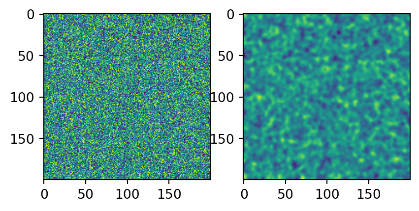

Comments

As we saw in the previous chapter, image analysis often involves nested for-loops to scan the pixels on each row and column. In this case of the gaussian_filter, 2 additional levels of for-loops are required since the neighborhood around each pixel must be scanned to get the ‘gaussian-weighted’ average of the neighbors. Not only does the Scipy implementation work faster, but it also implements something that we might find quite challenging to figure out.

9.5 Saving and Loading Numpy Arrays

Now that we are thoroughly comfortable with Numpy arrays it is likely that we’ll be using them for everything. This means we might want/need to save our data to disk for use later.

Numpy offers 2 convenient ways to do this.

9.5.1 Saving Single Arrays

arr = np.random.rand(100, 100)
1np.save('random_values', arr)

1: If we don’t include a file extension Numpy will add .npy for us.

And of course we can load it back from the disk into active memory just as easily:

1arr2 = np.load('random_values.npy')
print(np.all(arr == arr2))

1: We have to include the file extension when we load the file, otherwise Numpy won’t be able to find it because random_values and random_values.npy are both valid file names.

True

The np.save() and np.load() functions save the numerical data in binary format, meaning these files are not human readable. Numpy does offer savetxt and loadtxt to write/read normal text files, but this not recommended for saving large amounts of data since conversion to and from string slows everything down.

9.5.2 Saving Multiple Arrays

Often we are working on a project that has many arrays, such as processing a batch of images. We can save all these arrays to a single archive file. This helps with keeping related items together in one place.

arr1 = np.random.rand(100, 100)
arr2 = np.random.rand(100, 100)
1np.savez('multiple_random_arrays', foo=arr1, bar=arr2)

1: If we don’t specify a file extension Numpy will use .npz. The z reminds us that it’s an archive containing multiple files.

Now to read them back in we can use the same np.load() function, which will adapt to handle the archive instead of just a single array.

dict_containing_both_arrays = np.load('multiple_random_arrays.npz')

The function returns a “dict-like” object and we can access the arrays using the keywords that we used when we wrote the file:

1arr3 = dict_containing_both_arrays['foo']
print(np.all(arr1 == arr3))

1: We can access the saved array using the dictionary key corresponding to the keyword we used when we saved it.

True

Lastly, Numpy offers us a way to save an archive of files in a compressed format to save space. This is acomplished with np.savez_compressed(). The files are still reloaded using np.load(), and the reuslt is a dictionary like discussed above.

9.1 Broadcasting

9.1.1 Broadcasting: Rule 1

9.1.2 Broadcasting: Rule 2

9.1.3 Broadcasting: Rule 3

9.2 Ufuncs

9.2.1 Ufuncs that Operate on a Single Array

9.2.2 Ufuncs that Operate on Pairs of Arrays

9.3 Numpy’s Modules

9.3.1 The numpy.random Module

9.3.2 The numpy.linalg Module

9.3.2.1 matmul

9.3.2.2 Other Linear Algebra Functions

9.4 A Tour of Scipy

9.5 Saving and Loading Numpy Arrays

9.5.1 Saving Single Arrays

9.5.2 Saving Multiple Arrays

9.3.1 The `numpy.random` Module

9.3.2 The `numpy.linalg` Module

9.3.2.1 `matmul`