8  Numerical Computing Part 1: Introduction to Numpy

Figure 8.1: The feeling you get when something is 100x faster AND you wrote less code.

Although it might not always seem like it, Python is actually very easy to use (compared to other languages). Not only does it have a very readable syntax, but it also let’s us mix-and-match types with impunity. Python deals with the operations on different types “on-the-fly”. Consider the following case:

1a = [1, 1.0, '1', 'one', True, 1+0j]
for item in a:
2  b = item*2
  print(b)

1

We have a collection where every item has a different type

2

The item*2 operation does something different on each loop! Python has to check the type of item EVERY. SINGLE. TIME. This really slows things down.

2
2.0
11
oneone
2
(2+0j)

The slow-down incurred by having to check the type of each variable before doing an operation is quite problematic in numerical computing. Looping through large lists, vectors, arrays, and matrices of data is the basis for all numerical computations.

Example 8.1 (Invert an image) Given a greyscale image below, invert the colors so that dark becomes light, and vice-versa.

Figure 8.2: Smiley in black and white, aka greyscale.

Solution

Images are represented as 2D matrices with values between 0 and N indicating the color, where N=255 in this case. We can look at a small piece of the array to confirm:

import matplotlib.pyplot as plt
1im = plt.imread("media/smiley.jpg")[..., 0]
2print(im[200:210, 200:210])

1

The imread function fetches the image file and returns it as a numpy array, which we’ll learn about below.

2

Here we take a “slice” of the array to inspect the values in a small portion.

[[198 198 198 199 199 199 199 199 197 198]
 [198 198 198 199 199 199 199 199 197 198]
 [198 198 198 199 199 199 199 199 198 198]
 [198 198 198 199 199 199 199 199 198 198]
 [198 198 198 199 199 199 199 199 198 198]
 [198 198 198 199 199 199 199 199 198 199]
 [198 198 198 199 199 199 199 199 198 199]
 [198 198 198 199 199 199 199 199 198 199]
 [199 199 199 199 198 198 198 198 197 198]
 [199 199 199 199 198 198 198 198 198 199]]

To invert the greyscale values in im using traditional for-loops, we need to do 2 nested loops to scan along each row. Just for fun, let’s also record the time it takes to do this:

from time import time

tstart = time()

im2 = im.copy()
im_max = im.max()
for i in range(im.shape[0]):
    for j in range(im.shape[1]):
        im2[i, j] = im_max - im[i, j]

tfinal = time() - tstart
print(f"This took {tfinal} seconds")

This took 0.037322998046875 seconds

Now we can visualize the images side-by-side to confirm we achieved our objective:

fig, ax = plt.subplots(2, 1)
ax[0].imshow(im, cmap=plt.cm.bone)
ax[1].imshow(im2, cmap=plt.cm.bone)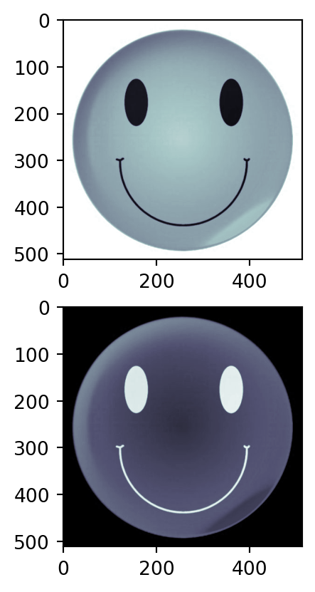

Comments

Note that indexing into this 2D numpy array is different than a 2D list.

• To get the first element of a 2D list we use arr[0][0]…we index into the “outer” list to get access to the “inner” list, so it’s like chaining the indices.
• To get the first element of a 2D numpy array we use arr[0, 0]. We access all the dimensions at the same time.

8.1 Introducing the ndarray

Note

numpy is not included in Python. We need to install it separately. If we used Anaconda to get ourselves started, then we get numpy included (along with a few hundred other packages). So despite the fact that numpy is pretty much mandatory for any numerical computing, it is still a separate package with its own “interface” that we must learn.

The main feature of numpy is a new data-type known as an ndarray. This array looks and acts a lot like a list but has one key difference:

Every item in an ndarray must be the same type!

This means that is is now possible to scan an ndarray without checking the type of each item, thus avoiding that slow process.

HOWEVER, it is not quite that simple. If we attempt to use Python for-loops to index into ndarrays Python will still check the type. However, numpy provides us with literally hundreds of functions that we can use to accomplish almost anything that would otherwise require for-loops.

The downside is that using numpy is like learning a language within a language.

Just In Time Compilation (JIT)

Probably 99% of the time we can get by using some combination of numpy functions and functionality, but if we are doing something really special the use of a for-loop may be necessary. In this case we can still avoid slow Python for-loops by using a package called numba. numba lets us write functions with for-loops to scan through ndarrays, but the loops are fast. This package basically provides a way to write a for-loop with avoids the type-checking of each item. It’s a bit of a pain to use though.

It uses a technique called “just in time” compilation, and it looks at the type of input data to the function, then compiles a version of the function that works on that data type only. This is another way to avoid type checking since it knows that the data received by the function is of one single type.

8.1.1 Data Type of an Array

Since each element in an ndarray is of the same type, then we shouldn’t be surprized that the ndarray itself has a type, and that type corresponds to the contents.

import numpy as np

1arr = np.array([1, 2, 3], dtype=int)

2print(type(arr))
3print(arr.dtype)

1

When creating an ndarray, we can optionally specify dtype, in this case int. dtype stands for “data type” and it limits which type of values can be stored within arr. The default is float.

2

If we do the normal type-check we will see that Python see this as an ndarray, which is it.

3

However, the ndarray itself has an “attribute” which tells us the type of the data inside arr. numpy gives us a bit more information that just int…it says int64 which means an integer represented using 64-bits, so is extra accurate.

<class 'numpy.ndarray'>
int64

We can create arrays with all the usual types:

arr2 = np.array([1, 2, 3], dtype=float)
print(arr2)
arr3 = np.array([0, 1, 0], dtype=bool)
print(arr3)
arr4 = np.array([1, 2, 3], dtype=complex)
print(arr4)

[1. 2. 3.]
[False  True False]
[1.+0.j 2.+0.j 3.+0.j]

You can also specify the number of bits to use, to manually balance higher accuracy (high bits) and lower memory usage (lower bits). Operations on arrays with lower bits are also faster since there is less “stuff” to compute. numpy includes these extra types, such as np.int8 and np.float128. We can confirm that they do take up different amounts space:

import numpy as np
arr2 = np.array([1, 2, 3], dtype=np.int8)
print(arr2.nbytes)
arr3 = np.array([1, 2, 3], dtype=np.int16)
print(arr3.nbytes)
arr4 = np.array([1, 2, 3], dtype=np.float64)
print(arr4.nbytes)

3
6
24

It is easy to convert between types using the astype() method attached to each ndarray:

arr = np.array([1, 2, 3])
arr = arr.astype(int)
print(arr)

[1 2 3]

8.1.2 Elementwise Operations

One of the ways that numpy let’s us avoid the use of for-loops is by changing they way mathematical operations like + and * work.

Recall that for lists, multiplication by 2 doubled the length of the list:

arr = [1, 2, 3] * 2
print(arr)

[1, 2, 3, 1, 2, 3]

With numpy, multiplication does actual math!:

import numpy as np
arr = np.array([1, 2, 3]) * 2
print(arr)

[2 4 6]

This is called “elementwise” operation because it operates on each element, rather than on the whole array.

numpy also allows for elementwise operations between 2 arrays:

arr1 = np.array([1, 2, 3])
arr2 = np.array([10, 20, 30])
print(arr1/arr2)

[0.1 0.1 0.1]

All mathematical operations are supported:

arr1 = np.array([1, 2, 3])
arr2 = np.array([4, 5, 6])
print( arr1 + arr2)
print( arr1 - arr2)
print( arr1 * arr2)
print( arr1 / arr2)
print( arr1 // arr2)
print( arr1 % arr2)
print( arr1**arr2)

[5 7 9]
[-3 -3 -3]
[ 4 10 18]
[0.25 0.4  0.5 ]
[0 0 0]
[1 2 3]
[  1  32 729]

In all cases, each of the above lines performs the stated operation using element i of arr1 and element i of arr2.

Note

When we perform elementwise operations with ndarrays what actually happens is that “behind the scenes” some special code is run which performs for-loops that do not check the type. In this way we can achieve much faster speeds.

Example 8.2 (Inverting an image using numpy) Let’s perform the same operation on “smiley” as in Example 8.1, but using numpy's elementwise mathematical features.

Solution

import matplotlib.pyplot as plt
from time import time

im = plt.imread("media/smiley.jpg")

1im = np.array(im)[..., 0]

tstart = time()

2im3 = im.max() - im

tfinal2 = time() - tstart
print(f"This took {tfinal2} seconds")

1

Here we convert im to an ndarray for demonstration purposes only, because in fact an ndarray is returned by the imread function already.

2

Because im is an ndarray the - operation will use numpy's elementwise operations.

This took 0.00015807151794433594 seconds

Comments

The speed-up we achieved was 234.63 times! The speed-up is almost always >50-100x. A 100x speedup is the difference between 36 seconds and one hour! Or 3 days and a year.

For-loops are OK sometimes

In the above example we used elementwise operations to perform an operation on an image, providing a huge speed-up. The lesson is that we should NOT use for-loops to process the individual elements a big array. However, it is still OK to use a for-loop to process a big batch of images, using numpy functions inside the loop, like this:

ims = [im1, im2, im3, im4, im5]
mx = []
for im in ims:
    mx.append(im.max()) 

The point is that looping over a small number of items and doing big calculations on each loop is fine, common, and usually unavoidable.

8.1.3 Array Properties

8.1.3.1 Attributes

When we looked at Python containers like lists and strings, we used the various methods that were attached to them. These methods are just functions which operate on the object, so vals.sort() is the same as sorted(vals).

ndarray also have a lot of methods attached to them, which we’ll cover later. They also have a lot of “attributes” attached to them. Attributes store information about the array, such as size and shape. A list of useful “attributes” on ndarrary is given below:

Table 8.1: List of commonly used attributes on ndarrays

Attributes	Description
ndim	Number of dimension of the array
size	Number of elements in the array
shape	The size of the array in each dimension
dtype	Data type of elements in the array
itemsize	The size (in bytes) of each elements in the array
data	The buffer containing actual elements of the array in memory
T	View of the transposed array
dict	Information about the memory layout of the array
flat	A 1-D iterator over the array
imag	The imaginary part of the array
real	The real part of the array
nbytes	Total bytes consumed by the elements of the array

The shape, size and ndim get used a lot, while the rest are mostly there for debugging.

import numpy as np

arr = np.array([[2, 3, 4], [3, 4, 5]])
print(arr.shape)
print(arr.size)
print(arr.ndim)

(2, 3)
6
2

8.1.3.2 Methods

Attributes discussed above are values which do not need to be computed, like arr.size. There are many other properties of an array which would like to know, such as the maximum or minimum value within it. This sort of information must be calculated on demand using the methods attached to the ndarrays.

arr = np.array([4, 3, 6])
print(arr.max())
print(arr.min())

6
3

Note that because these methods require an actual computation on the array, it is best to store their result if it needs to be used many times:

arr = np.array([4, 3, 6])
amax = arr.max()

Table 8.2: List of methods on ndarrays which calculate some property based on the array contents

Method	Description
max	Return the maximum along a given axis.
min	Return the minimum along a given axis.
trace	Returns the sum along diagonals of the array.
sum	Return the sum of the array elements over the given axis.
cumsum	Returns the cumulative sum of the elements along the given axis.
mean	Returns the average of the array elements along given axis.
var	Returns the variance of the array elements, along given axis.
std	Returns the standard deviation of the array elements along given axis.
prod	Returns the product of the array elements over the given axis
cumprod	Returns the cumulative product of the elements along the given axis.
all	Returns True if all elements evaluate to True.
any	Returns True if any of the elements of a evaluate to True.

Example 8.3 (Compute the cumulative sum of an array) Given a 1D array, compute the cumulative sum of all the values. Compare a for-loop with the ndarray method in terms of speed.

Solution

from time import time

arr = np.random.randint(0, 1000, 10000)

tstart = time()
csum = 0
for val in arr:
    csum = csum + val
 
tend1 = time() - tstart
print(f"The time required was {tend1} seconds")

The time required was 0.0004971027374267578 seconds

Now doing the same thing with ndarray.cumsum():

from time import time

arr = np.random.randint(0, 1000, 10000)

tstart = time()
csum = arr.cumsum()
 
tend2 = time() - tstart
print(f"The time required was {tend2} seconds")

The time required was 0.0001621246337890625 seconds

Using the numpy function resulted in a speed up of {python} round(tend1/tend2, 3).

Comments

This is example of how numpy provides us with a function which performs an operation which would otherwise require a for-loop.

By default all of the methods in Table 8.2 operate on all axes. For instance, max returns a single value which is the maximum value for the entire array. Most of these methods also accept an axis argument, in which case a new ndarray is returned which is one dimension smaller than the original array, containing the result obtained by only looking at values along a given axis.

Example 8.4 (Analyze array along a given axis) You have weather data for a half a day, in the form of a CSV file. Each column contains a different piece of meteorological data, like temperature and humidity. Each row represents the point in time at which the data were measured (one per hour). Find the average value of each column for the day.

t	T	RH
0	12	75
1	12	75
2	11	75
3	11	77
4	10	77
5	10	79
6	11	78
7	12	76
8	14	72
9	16	72
10	19	70
11	20	65
12	20	65

Solution

# After reading the data from CSV file we have the following:
data = [[0,  12, 75],
        [1,  12, 75],
        [2,  11, 75],
        [3,  11, 77],
        [4,  10, 77],
        [5,  10, 79],
        [6,  11, 78],
        [7,  12, 76],
        [8,  14, 72],
        [9,  16, 72],
        [10, 19, 70],
        [11, 20, 65],
        [12, 20, 65]]
1data = np.array(data)
2aves = data.mean(axis=0)
print(aves)

1

We need to convert to an ndarray first

2

Once we have an ndarray we can call the desired method with the axis as an argument

[ 6.         13.69230769 73.53846154]

Comments

By default axis=None, which means that the mean for the entire array is found. This does not make sense since the data in each column are totally unrelated.

8.1.4 Multidimensional Arrays and Indexing

Multidimensional arrays are very common in numerical programming. Some examples are:

1. A greyscale image is a 2D array as we saw in Example 8.2.
2. A color image is actually 3D. At each pixel in the 2D view, there is an extra dimension containing the “RGB” values, which dictate the proportion of red, blue, and green to show at that location. So a 2D color image would have dimensions like [200, 200, 3].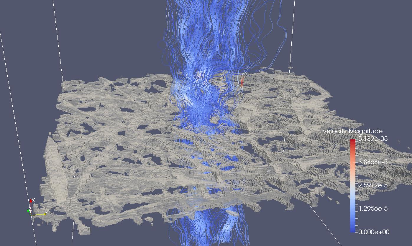
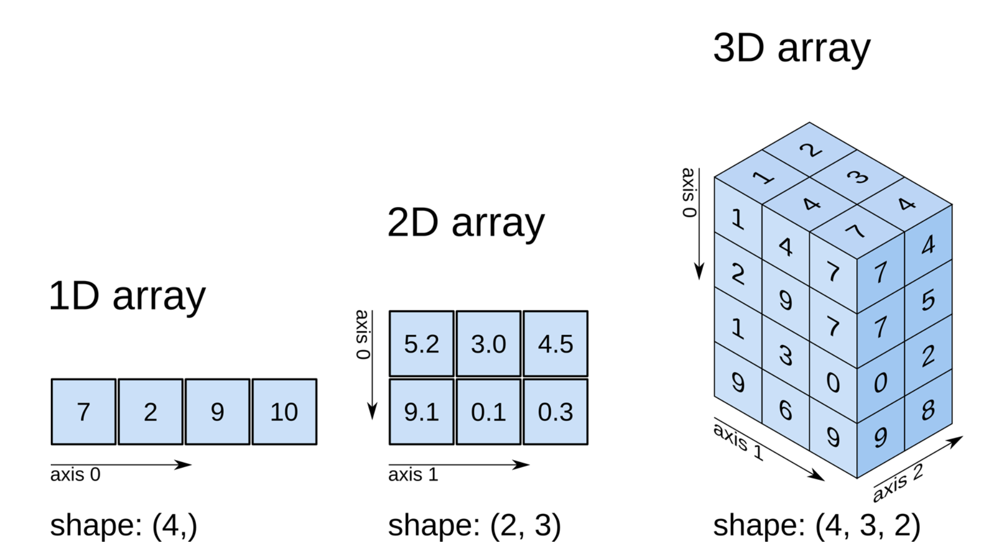
3. A greyscale video is a 3D array. Each moment in time (a frame) is a 2D array, and time is the third axis. Of course, if the video is color, this requires an extra dimension.
4. 3D images are common in medical applications, such images are produced by x-ray tomography (i.e. cat-scans) and MRI scans. These can be though of as a stack of 2D slices.

Figure 8.3: Fluid flow simulation through a 3D image of a fibrous electrode

As “simple humans” we can visualize 1D, 2D and 3D images and arrays quite well, but not higher. Figure 8.5 shows this progression. It also includes the definition of array “shape” as well:

Figure 8.4: Schematic visualization of 1D, 2D and 3D arrays

Note

It is actually possible to use the “list of lists” style indexing with ndarrays, as shown below:

import numpy as np

arr = np.random.rand(5, 5)
print(arr[0][0])
print(arr[0, 0])

0.2977770674188823
0.2977770674188823

But numpy offers several special features which require the [0, 0] style indexing, so it’s necessary to learn this. For instance, we can extract a subsection of an array using:

import numpy as np

arr = np.random.rand(9, 9)
arr2 = arr[:3, :3]
print(arr2)

[[0.08277747 0.7282641  0.79949882]
 [0.79218985 0.45573028 0.80296608]
 [0.3168688  0.56676578 0.97257359]]

8.1.4.1 Indexing ndarrays

Indexing an ndarray behaves a bit differently than we have seen with nested lists. Recall that indexing into a nested list (i.e. a “list of lists”) worked as follows:

lol = [[1, 2, 3],
       [4, 5, 6],
       [7, 8, 9]]
1print(lol[0])
2print(lol[0][0])

1

If we use a single index, [0], we retrieve the list stored at location 0.

2

By adding a second [0] we index into the list we obtained from the first [0].

[1, 2, 3]
1

For an ndarray, the indexing is done within a single pair of brackets:

arr = np.array([[1, 2, 3],
                [4, 5, 6],
                [7, 8, 9]])
1print(arr[0, 0])

1

Here we specify the row and col simultaneously and receive the value stored at that location.

1

Visualizing 4D and higher becomes a challenge. Humans are fundamentally incapable of visualizing higher dimension, so we need some tricks, as illustrated in the following example.

Example 8.5 (Thinking about higher dimensional arrays) Consider the array shown in Figure 8.5. How would you access the value of “31”?

Figure 8.5: Schematic diagram visualizing how to think about ND arrays

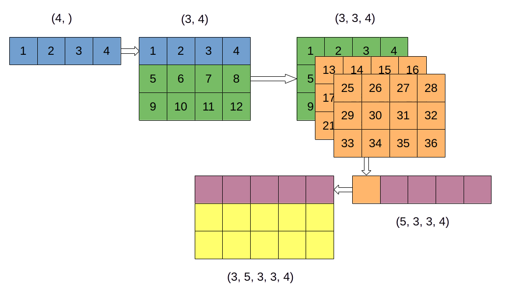
Solution

1arr = np.arange(1, 3*5*3*3*4 + 1)
2arr = arr.reshape([3, 5, 3, 3, 4])
3val = arr[0, 0, 2, 1, 2]
print(val)

1

Make a 1D array of values from 1 to N+1, where N is the total number of elements in the final array

2

Reshape the array into a 5 dimensional array

3

To access the specific value, we know it lies on the

31

Comments

numpy uses “C” ordering, which means that each new axis gets added to the beginning of the of list of axes. In other words, the highest dimension is indexed using the first index, and lowest dimension is last. Technically, this means that indexing is like arr[z, y, x], although it should be stressed that numpy does not name these axes. In fact, numpy calls these axes 0, 1 and 2 which is a bit counter-intuitive.

The alternative to “C” ordering if “F” ordering, referring to FORTRAN, where new dimensions are added to the end of the list of axes.

It is sometimes helpful to think of multidimensional arrays as being reshaped to 1D arrays. In fact, this is how computers “think” about. The values are laid out 1D block in memory. We can change the shape of any array as follows:

arr = np.arange(24)
print(arr)

[ 0  1  2  3  4  5  6  7  8  9 10 11 12 13 14 15 16 17 18 19 20 21 22 23]

arr = arr.reshape([4, 6])
print(arr)

[[ 0  1  2  3  4  5]
 [ 6  7  8  9 10 11]
 [12 13 14 15 16 17]
 [18 19 20 21 22 23]]

arr = arr.reshape([2, 12])
print(arr)

[[ 0  1  2  3  4  5  6  7  8  9 10 11]
 [12 13 14 15 16 17 18 19 20 21 22 23]]

We can swap between any shapes as long as the total number of elements is conserved.

8.1.4.2 Slicing an Array

We can also retrieve subsections of an array using “slicing” that we discussed in the previous chapter:

arr = np.arange(25)
arr = arr.reshape([5, 5])
print(arr)
print(arr[0:3, 0:3])

[[ 0  1  2  3  4]
 [ 5  6  7  8  9]
 [10 11 12 13 14]
 [15 16 17 18 19]
 [20 21 22 23 24]]
[[ 0  1  2]
 [ 5  6  7]
 [10 11 12]]

We can also write to subsections of an array:

arr = np.arange(25)
arr = arr.reshape([5, 5])
arr[0:3, 0:3] = 0
print(arr)

[[ 0  0  0  3  4]
 [ 0  0  0  8  9]
 [ 0  0  0 13 14]
 [15 16 17 18 19]
 [20 21 22 23 24]]

The defaults also apply, so we can omit some values:

arr = np.arange(25)
arr = arr.reshape([5, 5])
1arr[:3, 3:] = 0
print(arr)

1

Here we slice the first 3 rows from the start, and then from the 3rd column to the end. Remember that when using slice indexing, the start point is included but the stopping point is not, so :3 means the first 3 rows (0, 1 and 2), but does not include row 3.

[[ 0  1  2  0  0]
 [ 5  6  7  0  0]
 [10 11 12  0  0]
 [15 16 17 18 19]
 [20 21 22 23 24]]

8.1.4.3 Masking

As with mathematical functions, logical comparisons are also done elementwise:

import numpy as np

1arr = np.random.rand(5, 5)
2mask = arr < 0.5
3print(mask)

1

Generate a 5x5 array of random numbers between 0 and 1.0

2

Perform a logical comparison to determine which values in arr are less than 0.5

3

Printing mask reveals that it contains True and False values, which are the result of the logical comparison.

[[ True  True False False  True]
 [False False False False False]
 [ True False  True  True  True]
 [ True  True  True False False]
 [ True False False  True False]]

We can use ndarrays filled with boolean values as “masks” to retrieve or write values from the locations where the mask is True.

import numpy as np

arr = np.random.rand(5, 5) 
1mask = arr < 0.1
2vals = arr[mask]
print(vals)

1

mask will contain a True value in all locations where arr < 0.1.

2

We can retrieve all the values in arr that were < 0.1 using mask for the index.

[0.04582099 0.03236906 0.03972382]

We can also use masks to write values:

import numpy as np

arr = np.random.rand(5, 5)
mask = arr < 0.5
1arr[mask] = 0.0
print(arr)

1

Here we tell numpy to put the value of 0.0 into arr at all locations where mask is True.

[[0.         0.74978164 0.         0.         0.94784757]
 [0.52248844 0.         0.         0.56699272 0.90824512]
 [0.         0.         0.         0.         0.        ]
 [0.74340212 0.58336774 0.94278052 0.6906021  0.        ]
 [0.58078615 0.99266985 0.90875989 0.         0.5816829 ]]

Example 8.6 (Use masking to write many values to an array) Find all values in a array of random numbers less than 0.5, and replace them with the negative of their square root.

Solution

import numpy as np

arr = np.random.rand(5, 5)
mask = arr < 0.5
1new_vals = -arr[mask]**0.5
2arr[mask] = new_vals
print(arr)

1

new_vals is a 1D array of values computed as request

2

Here we insert the items from the new_vals array into arr.

[[-0.41487194 -0.59249896  0.76346152  0.8076029   0.85005044]
 [-0.51017919  0.70484376 -0.55813356 -0.28462852 -0.67151771]
 [-0.70391373  0.59912519 -0.62340493  0.56605383  0.78497231]
 [ 0.89299266 -0.31350605  0.63552144 -0.27002183 -0.49324984]
 [ 0.88100151  0.8927954  -0.22843895 -0.62728611 -0.63428898]]

Comments

The key thing to note in the above code is that both the operations where mask is used return a 1D array. So even though arr was a 5-by-5 ndarray, the operations are all done on a “flattened” version of size 25-by-1.

print(new_vals)

[-0.41487194 -0.59249896 -0.51017919 -0.55813356 -0.28462852 -0.67151771
 -0.70391373 -0.62340493 -0.31350605 -0.27002183 -0.49324984 -0.22843895
 -0.62728611 -0.63428898]

and

print(arr[mask])

[-0.41487194 -0.59249896 -0.51017919 -0.55813356 -0.28462852 -0.67151771
 -0.70391373 -0.62340493 -0.31350605 -0.27002183 -0.49324984 -0.22843895
 -0.62728611 -0.63428898]

8.1.4.4 Fancy Indexing

Fancy indexing works like the masks discussed above for masks, but with actual numerical index values:

import numpy as np

1arr = np.random.rand(10)
2indices = [0, 4, 8, 5]
3arr[indices] = 0.0
print(arr)

1

Here we are working with a 1D array since it’s simpler

2

We can create a list of numerical index values, and they do not have to be in order

3

Lastly, we use the indices to write a value to each given location.

[0.         0.08517893 0.19606165 0.26219769 0.         0.
 0.47375759 0.72581009 0.         0.84949167]

When working with higher-dimensional arrays (2D, 3D, etc), we must specify the index of each axis in its own list (like above for 1D), but then combine each list in a tuple:

import numpy as np

arr = np.random.rand(5, 5)
ind_x = [0, 0, 1, 3, 3]
ind_y = [0, 1, 3, 3, 4]
indices = (ind_x, ind_y)
arr[indices] = 0.0
print(arr)

[[0.         0.         0.1474802  0.33153472 0.21024793]
 [0.14531768 0.19587551 0.56404873 0.         0.85686775]
 [0.91742026 0.9183996  0.7044764  0.26802012 0.46294791]
 [0.82980378 0.75089697 0.51382404 0.         0.        ]
 [0.03311313 0.85773795 0.05355766 0.87403983 0.72244447]]

Example 8.7 (Using the where function) Give an array of random numbers between 0 and 1, find all the locations where the value is less than 0.5 and replace them with 2x the value.

Solution

import numpy as np

arr = np.random.rand(5, 5)
mask = arr < 0.5
1indices = np.where(mask)
arr[indices] = 2*arr[indices]
print(arr)

1

where is one of the many functions that numpy offers. It returns the indices of the locations where a condition is met. It returns the indices as lists for each axis, combined in a tuple, so the result is ready for direct use for fancy indexing.

[[0.97877883 0.30634607 0.87586577 0.24342061 0.99619964]
 [0.75267402 0.81460794 0.44593243 0.08835558 0.95475941]
 [0.10256801 0.20526574 0.53322036 0.9440505  0.57694484]
 [0.629568   0.9243888  0.08658308 0.79334562 0.3968679 ]
 [0.78395268 0.35373901 0.45972695 0.50161711 0.86732623]]

Comments

8.2 Creating Numpy Arrays

In all of the above code snippets and examples we have seen that ndarrays can be created by lists as follows:

vals = [1, 2, 3, 4, 5]
arr = np.array(vals, dtype=int)
print(arr)

[1 2 3 4 5]

It is also possible to convert an ndarray back to a list:

vals = [1, 2, 3, 4, 5]
arr = np.array(vals, dtype=int)
vals2 = arr.tolist()
print(type(vals2))

<class 'list'>

Often we want to create an ndarray directly. We can create an empty array with a given shape and type:

arr = np.ndarray(shape=[5, 2])
print(arr)

[[0.         0.08517893]
 [0.19606165 0.26219769]
 [0.         0.        ]
 [0.47375759 0.72581009]
 [0.         0.84949167]]

Note that the above array was filled with gibberish. These values are the numerical representation of whatever leftover data was stored in the memory that was assigned to hold arr. It is probably more useful to create an array of 1’s or 0’s, so numpy provides functions for that:

arr1 = np.ones(5, dtype=int)
arr2 = np.zeros(5, dtype=int)
print(arr1)
print(arr2)

[1 1 1 1 1]
[0 0 0 0 0]

8.3 Splitting and Joining Arrays

Often we want to combine two 1D arrays into a 2D array, or vice versa. numpy uses the term “stack” to refer to joining arrays. This refers to the fact that arrays “stack” like blocks, either beside or on top of each other.

Example 8.8 (Using hstack) Given 3 separate arrays that contain the x, y and z coordinates of of N points, join them into a single N-by-3 array.

Solution

N = 10
x, y, z = np.random.rand(3, N)

Let’s inspect the shape of these individual arrays:

print(x.shape)

(10,)

We can “stack” these vertically as follows:

coords = np.vstack((x, y, z))
print(coords.shape)

(3, 10)

This array is not the requested shape, but we can get the transpose using T:

coords = coords.T
print(coords.shape)

(10, 3)

Comments

Had we used hstack instead of vstack we would not have received the correct shape either:

coords = np.hstack((x, y, z))
print(coords.shape)

(30,)

In this case it just created a single long array.

If we wanted to create the N-by-3 array directly we would need to reshape x, y, and z first. We’ll turn each array into a vertical array, then stack them horizontally:

x = x.reshape([10, 1])
y = y.reshape([10, 1])
z = z.reshape([10, 1])
coords = np.hstack((x, y, z))
print(coords.shape)

(10, 3)

The above various and nuances are why using numpy is like learning a language within a language.

Splitting arrays into smaller ones is also fairly common. We have already seen that slice indexing can be used for this, such as:

arr = np.arange(16).reshape([4, 4])
a1 = arr[:2, :]
a2 = arr[2:, :]
print(a1)
print(a2)

[[0 1 2 3]
 [4 5 6 7]]
[[ 8  9 10 11]
 [12 13 14 15]]

However, it is often more convenient to use numpy's built-in functions. This makes it less likely to make mistakes for instance, and it’s also fewer lines of code:

arr = np.arange(16).reshape([4, 4])
1a1, a2 = np.vsplit(arr, 2)
print(a1)
print(a2)

1

This splits the array vertically, at row 2.

[[0 1 2 3]
 [4 5 6 7]]
[[ 8  9 10 11]
 [12 13 14 15]]