a, *b = 1, 2, 3
print('a is:', a)
print('b is:', b)
a is: 1
b is: [2, 3]After this lesson you should…
set collection and its special featureslist and dict comprehensions in place of simple for-loops, including if-clausesenumerate over a collection, as well as zip multiple collections together
When Guido created Python he was partly motivated by the realization that code is read more often than it is written. With this insight in mind he created a syntax that was as close to spoken English as possible. We have seen examples of this with statements like for item in collection. When code is written in a clean, concise, and consistent manner it becomes easy to read your own code as well as someone elses. Writing clean code is called “pythonic code”.
Pythonic code means two things. First is that the formatting of the code follows the standard conventions:
find_roots, instead of findroots, FindRoots or findRoots.x = 1 instead of x=1.To facilitate nice and consistent code, there is a style guide generally referred to as pep8.
The Python community created a process where new features can be proposed for the language. These proposals are called “peps”, an acronym for “Python Enhancement Proposal”. A list of all proposals is available, along with whether they have been accepted, rejected or are in progress. They are numbered, starting from 001, and we are now up to around 800.
The second aspect of Pythonic code is how the code is written, meaning the method used for certain common tasks uses the features of Python to their fullest. Examples include:
in keyword for checking membership and scanning over collections, like if item in collection or for item in collection.try/except blocks to do checking of type and general validity.PEP8 was created very early on, and has been a core part of Python ever since. This PEP basically describes how Python code should look. A condensed version of this guide, including examples is given here.
Why is it truly important to format your code?
| Readability | Formatting your code will help you read your code efficiently. It looks more organized, and when someone looks at your code they’ll get a good impression. |
| Coding Interviews | When you’re in a coding interview, sometime the interviewers will care if you’re formatting your code properly. If you forget to do that formatting you might lose your job prospects, just because of your poorly formatted code. |
| Team Support | Formatting your code becomes more important when you are working in a team. Several people will likely be working on the same software project and code you write must be understood by your teammates. Otherwise it becomes harder to work together. |
| Easier to spot bugs | Badly formatted code can make it really, really hard to spot bugs or even to work on a program. It is also just really horrible to look at. It’s an offense to your eyes. |
Here are a few highlights:
Instead of listing off all the rules, the following table demonstrates several (but not all):
| Yes | No |
|---|---|
spam(ham[1], {eggs: 2}) |
spam( ham[ 1 ], { eggs: 2 } ) |
if x == 4: print x, y; x, y = y, x |
if x == 4 : print x , y ; x , y = y , x |
spam(1) |
spam (1) |
dct['key'] = lst[index] |
dct ['key'] = lst [index] |
i = i + 1 |
i=i+1 |
submitted += 1 |
submitted +=1 |
x = x*2 - 1 |
x = x * 2 - 1 |
hypot2 = x**2 + y*y |
hypot2 = x ** 2 + y * y |
c = (a+b) * (a-b) |
c = (a + b) * (a - b) |
c = (a+b) / (a-b) |
c = (a + b)/(a - b) |
def complex(real, imag=0.0): |
def complex(real, imag = 0.0): |
return magic(r=real, i=imag) |
return magic(r = real, i = imag) |
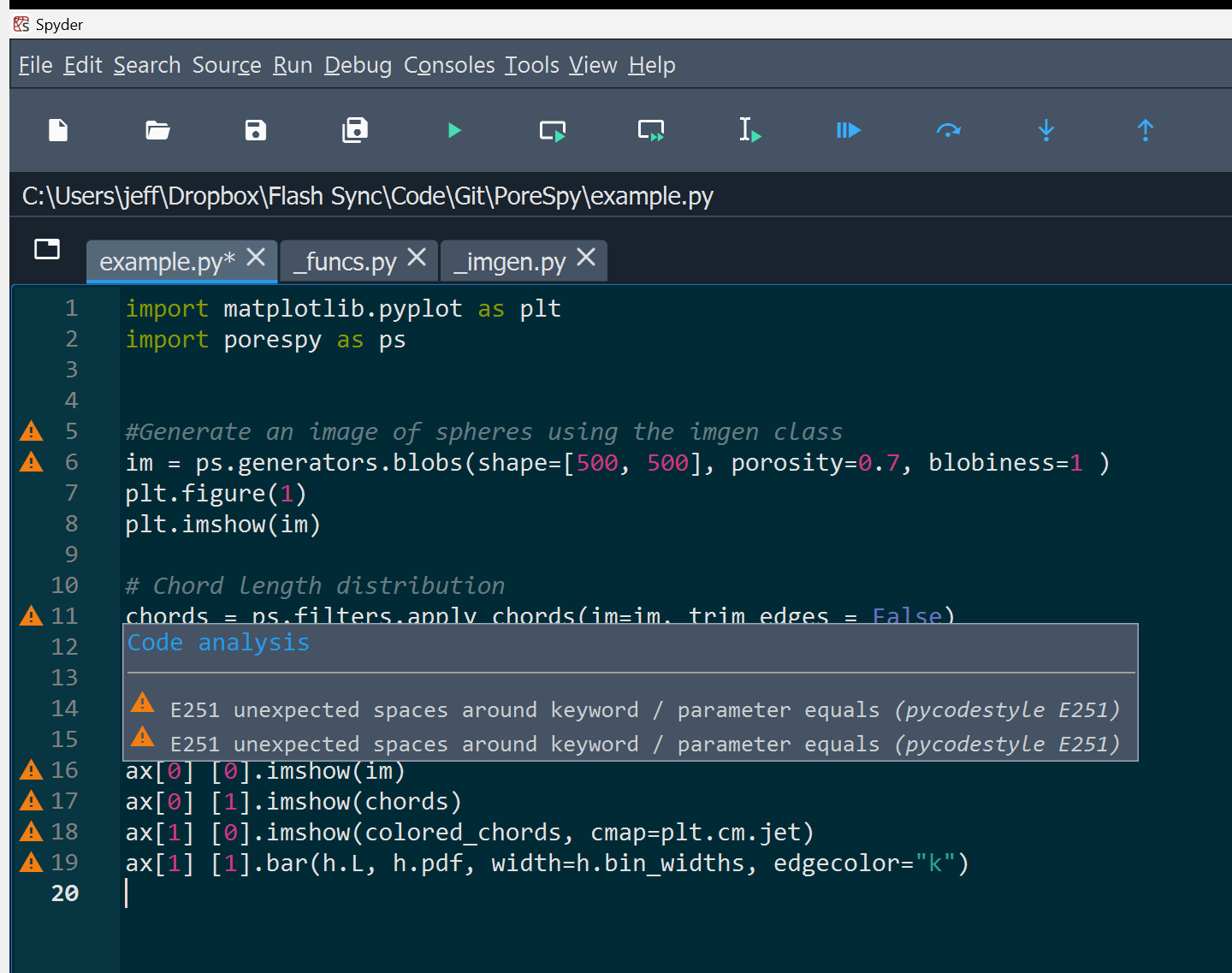
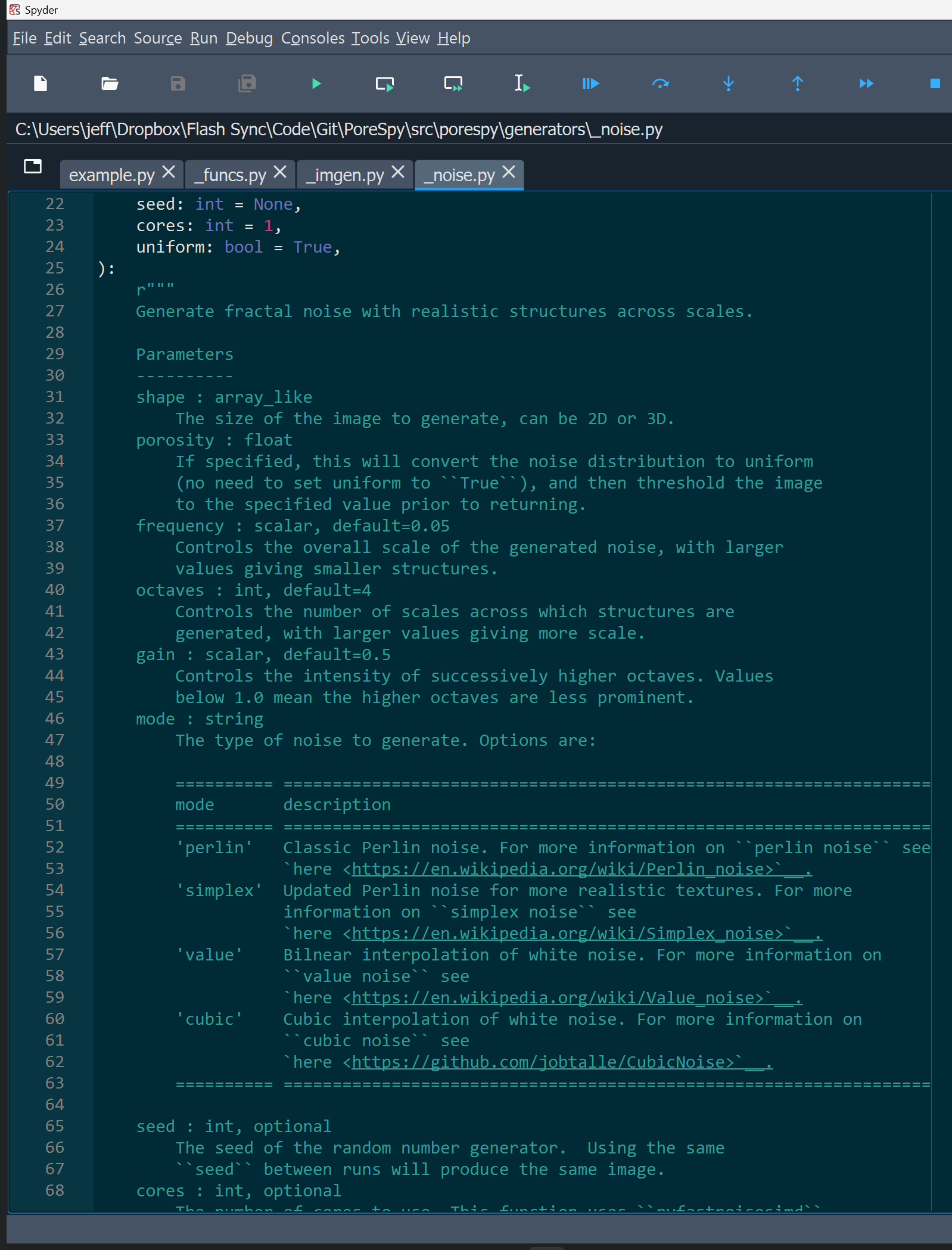
Since there are so many rules, it takes quite a while to learn them all. Luckily, there is a tool we can use called a linter. In IDE’s such as Spyder and VSCode it is possible to enable linting using a plugin or optional feature. The result looks like this:
As we will see below when looking at functions in more detail, Python allows us to unpack values in a collection into separate variables. This is sometimes called the “splat” operator.
a, *b = 1, 2, 3
print('a is:', a)
print('b is:', b)a is: 1
b is: [2, 3]We can even catch several individual values, and splat the rest into a single variable.
a, *b, c = 1, 2, 3, 4
print('a is:', a)
print('b is:', b)
print('c is:', c)
a is: 1
b is: [2, 3]
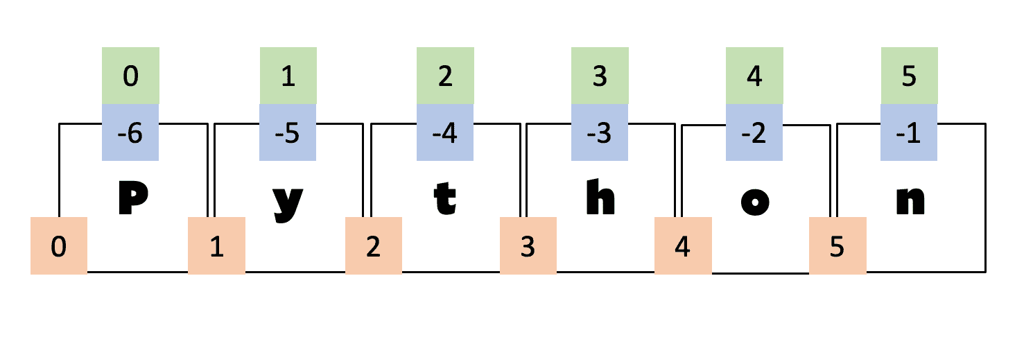
c is: 4We briefly covered slicing, but it will come up a lot more when we start to talk about numpy, so let’s take a closer look. We can use the : symbol to indicate a range of indices.
It works like this: start:stop:step. The default is 0:None:1, which means start at element 0, stop at the end indicated by None, and take steps of size 1. Since None does “nothing” you can also write 0::1.
Using the defaults gets us the entire list:
a = [0, 1, 2, 3, 4, 5, 6, 7, 8, 9]
1b = a[:]
print(b): alone will give the whole list. It is like writing [0:-1]
[0, 1, 2, 3, 4, 5, 6, 7, 8, 9]We can change the start and stop values to get a section of the list:
a = [0, 1, 2, 3, 4, 5, 6, 7, 8, 9]
1b = a[2:6]
print(b)6, not at 6.
[2, 3, 4, 5]The end point can be specified as distance from the start, or distance from the end by using a negative number:
a = [0, 1, 2, 3, 4, 5, 6, 7, 8, 9]
1b = a[2:-3]
print(b)2 and stop at 3 from the end.
[2, 3, 4, 5, 6]Changing the step size is also possible if we want every Nth item:
a = [0, 1, 2, 3, 4, 5, 6, 7, 8, 9]
1b = a[2:8:2]
print(b)[2, 4, 6]And of course the step can be negative if we want to walk through the collection backwards:
a = [0, 1, 2, 3, 4, 5, 6, 7, 8, 9]
1b = a[6:2:-1]
print(b)[6, 5, 4, 3]The final type of collection is called a set. This word is referring to the mathematical concept of a set. A set behaves similarly to a list (and therefor a tuple) with the defining feature being that it contains no duplicate elements.
A set is defined by putting curly braces around a comma-separated sequence of values:
1s = {1, 2.0, 'text'}
print("Result:", type(s))dict. The difference is that the collection only contains values, wheres in a dict it contains key:value pairs. There is actually some logic behind this: a set cannot contain any duplicate items, and similarly a dict cannot contain any duplicate keys. So {'a': 1, 'a': 2} will become {'a': 2}.
Result: <class 'set'>Python also includes a built-in function for creating sets:
1s = set([1, 2.0, 2.0, 2.0, 'text'])
print("Result:", s)2.0, yet the resulting set only has one instance.
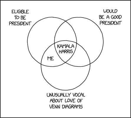
Result: {'text', 1, 2.0}Probably the most useful application of sets is for “Venn-diagram” style logic. For instance, if you have two lists of values, you might want to know what they have in common, or what are their differences. This can be accomplished with sets.
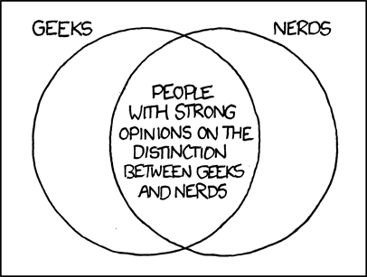
Consider the following 2 sets:
a = {'bob', 'dave', 'jane'}
b = {'dave', 'sue', 'taylor'}
We can find what the two sets have in common by finding the intersection:
a = {'bob', 'dave', 'jane'}
b = {'dave', 'sue', 'taylor'}
c = a.intersection(b)
print("Result:", c)
Result: {'dave'}Or we can find how they differ using difference:
a = {'bob', 'dave', 'jane'}
b = {'dave', 'sue', 'taylor'}
c = a.difference(b)
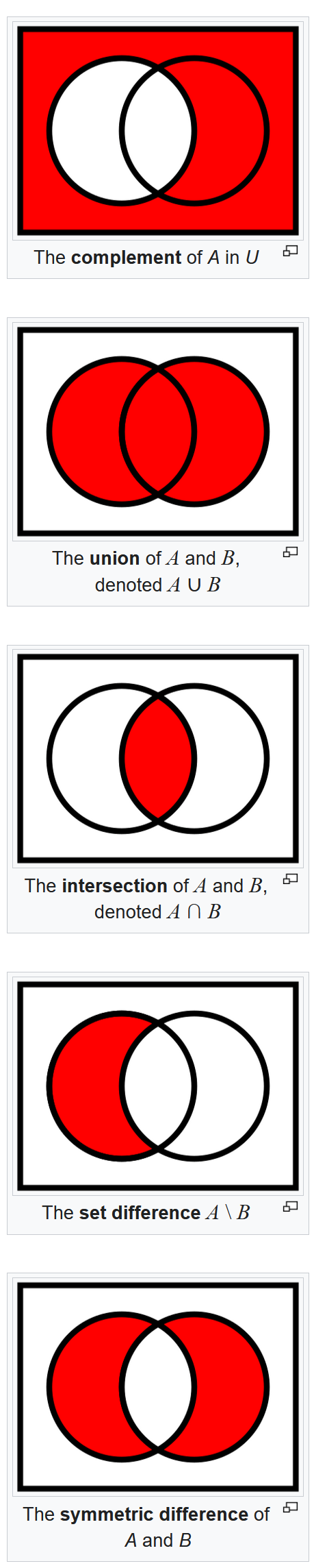
print("Result:", c)Result: {'jane', 'bob'}Table F.1 gives a list of the methods available on a set object which can be used for performing a variety of other “set operations” such those shown in Figure 7.5. An abbreviated list is given below with just the ones associated with “Venn-diagram”-type logic.
set object, including the shortcut keys which have been defined
| Method | Shortcut | Description |
|---|---|---|
difference() |
- |
Returns a set containing the difference between two or more sets |
intersection() |
& |
Returns a set, that is the intersection of two other sets |
issubset() |
<= |
Returns whether another set contains this set or not |
< |
Returns whether all items in this set is present in other, specified set(s) | |
issuperset() |
>= |
Returns whether this set contains another set or not |
> |
Returns whether all items in other, specified set(s) is present in this set | |
symmetric_difference() |
^ |
Returns a set with the symmetric differences of two sets |
union() |
| |
Return a set containing the union of sets |
We have seen For-Loops which iterate over the items in a collection:
c = ['a', 'b', 'c']
for item in c:
    print(item)
a
b
cAnd we have seen For-Loops which using an index into a collection:
c = ['a', 'b', 'c']
for i in range(len(c)):
    print(c[i])
a
b
cBut we can do both!
c = ['a', 'b', 'c']
for i, item in enumerate(c):
    print(i, item)
0 a
1 b
2 cHaving access to the item and to the index where is located is quite useful:
c = [22, 33, 44]
for i, item in enumerate(c):
    c[i] = item/11
print(c)
[2.0, 3.0, 4.0]We sometimes have 2 collections which we want to scan together, for example to combine the values into a dict. We can use the zip function as follows:
names = ['a', 'b', 'c']
nums = [1, 2, 3]
d = {}
for key, value in zip(names, nums):
    d[key] = value
print(d)
{'a': 1, 'b': 2, 'c': 3}We have been mostly looking at linear collections like lists and strings. However, we often have “multidimensional” data, like a “list of lists”. In such cases we need to use one for-loop to scan over the “outer” list, then a second for-loop to scan each “inner” list.
Another way to think about this is a 2D (or ND!) array of data, where one for-loop scans each row, then the second loop scans the columns of each row. Consider the following case of a 5-by-5 matrix:
Python prides itself on being easy to read. Often this means using as few lines as possible so that logic can be read as pseudo-sentence. It therefore offers an alternative way to write for-loops in a single line:
result = [item/4 for item in [-1, 0, 2, 3]]
print("Result:", result)
Result: [-0.25, 0.0, 0.5, 0.75]Technically this is called a list comprehension. They can be confusing at first, but eventually you may appreciate the conciseness they offer. It often helps readability to condense logic to a single line.
In addition to comprehensions with lists, we can also do dicts and tuples.
Dictionary comprehensions are helpful for combining two different data sources into a single dictionary. For instance if we have a list of names, and another list of values, we can do:
name = ['a', 'b', 'c', 'd', 'e']
data = [1, 2, 3, 4, 5]
1d = {name[i]: data[i] for i in range(len(data))}
print(d)dict, like d = {'a': 1, 'b': 2, 'c': 3}.
{'a': 1, 'b': 2, 'c': 3, 'd': 4, 'e': 5}The reason this is helpful is that we can effortlessly look up the value associated with 'c' as:
val = d['c']If this information were stuck in the list format, we’d have to do an extra step:
i = name.index('c')
val = data[i]
print(val)3The dict comprehension thus lets us combine the two lists into a single dict, and makes it simple to retrieve values corresponding to each name.
Since comprehensions are just For-Loops, they also work with zip and enumerate too:
name = ['a', 'b', 'c', 'd', 'e']
data = [1, 2, 3, 4, 5]
d = {k: v for k, v in zip(name, data)}
print(d)
{'a': 1, 'b': 2, 'c': 3, 'd': 4, 'e': 5}Recall the “One-line If-Statement”:
limit = 5
value = 'a' if 4 < limit else 'b'
print(value)aWe can combine this if condition in comprehensions too:
vals = [1, 2, 3, 4]
limit = 3
1a = [i for i in vals if i < limit]
print(a)if <comparison> at the end of this line does exactly what it implies linguistically. You can (almost) read this statement and know what it does.
[1, 2]In previous weeks we have discussed the differences between types and how Python tries to treat each variable accordingly. However, sometimes this just isn’t possible for Python and an error occurs. So far we have focused our energy on trying to intercept the variables and decide how to treat each one, but Python offers a way to handle this: try and except.
The basic idea is that we try to run some code first, and only if it fails do we do something else.
try:
    c = a + b
except:
    print('a and b are not compatible')
Let’s look at an example:
There are more “clauses” we can add to a try-except block. We can add an else which get run if there was no exception, and we can add a finally block, which get’s run no matter what:
try:
       # Some code which will usually run
except:
       # Handling of exception if required
else:
       # Execute if no exception
finally:
       # Some code that is always executed
These extra clauses are not very common, but are mentioned so if/when you see them in the wild, you’ll know what you’re seeing.
We have written a lot of functions in this class, but so far have not really extended their capabilities.
To start with, let’s identify the difference between position and keyword arguments. Consider the following function:
def add_values(a, b):
    return a + b
We can call it using positional arguments:
c = add_values(2, 2)Or keyword arguments:
c = add_values(a=2, b=3)When using keywords we can do this:
1c = add_values(b=3, a=2)a=2 onto a and b=3 onto b.
Lastly, note that positional arguments must come first, and then keyword arguments can follow:
c = add_values(2, b=3)In many functions there are some arguments which we don’t usually want to change. An example is something like mode='encrypt'.
This can be done in the function definition as follows:
def add(a, b, mode='normal'):
    if mode == 'normal':
        d = a + b
    elif mode == 'absolute':
        d = abs(a) + abs(b)
return d If you have a list or tuple of values, such coefficients (e.g. [1, 3, 5]), that you want to pass into a function, you can do the following:
def func(a, b, c):
    print(a, b, c)

vals = [1, 3, 5]
1func(*vals)* (asterisk) tells python to unpack the values in vals and place them into a, b, and c of the function. Obviously, the length of vals has to match the number of arguments in func.
1 3 5And taking this to the next level, we can use dicts as keyword arguments, where the key corresponds to the argument name.
def func(a, b, c):
    print(a, b, c)

vals = {'a': 1, 'c':5, 'b': 3}
1func(**vals)** (double asterisk) tells python to unpack vals and match up the keys with the arguments names, and pass the corresponding value from the dictionary, so the value in vals['a'] (1) gets passed to a. Obviously, the keys in vals have to match the number and names of the arguments in
1 3 5This functionality is important because there are many packages where functions are designed to work together. In the next example we’ll jump ahead to scipy.stats to see a use case for this.
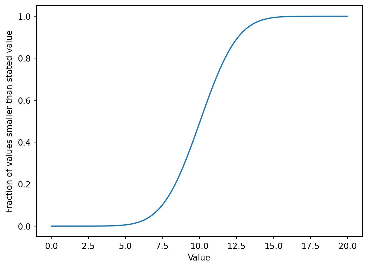
Example 7.6 (Using results from one function as arguments to another) Consider that we have a long list of data points, such as average weight of a pumpkin, and we want to fit a normal distribution to them. We will start by generating 1000 (artificial) data points with a mean value of 10 and a deviation of 2:
import numpy as np

data = np.random.normal(size=1000, loc=10, scale=2)
Solution
Now let’s use the functions in the scipy.stats module to fit a normal distribution to our data:
from scipy import stats

params = stats.norm.fit(data)
print(params)
(np.float64(10.01217183552977), np.float64(1.9974034202098299))Finally, let’s plot a graph of the cumulative distribution curve using the values of params we found above:
scipy.stats.norm to generate y values for the given x values using the params we found for this particular dataset.
matplotlib library which we’ll cover in more detail in a few chapters
Comments
Plotting data is a huge part of why we crunch numbers on a computer. There are a lot of libraries for plotting in Python, each has their own angle, but matplotlib is the OG. Everyone else needs to justify why you should use their library rather than matplotlib. Below is a list of the more popular ones, some of which we’ll revisit later.
We are now quite familiar with writing our own functions. We also also well aware that some functions can be complicated, and often need to be explained. This is what “docstrings” are for.
A basic (i.e. minimal) docstring is added to a function as follows:
def calc_area_and_perimeter(r):
1    r"""
2    Computes the area and perimeter of a circle

3    Parameters
4    ----------
5    r : scalar
6        The radius of the circle

7    Returns
    -------
    result : tuple of floats
        A tuple containing the area and perimeter, in that order
    """
8    A = 3.14159*(r)**2
    P = 2*3.14159*r
return (A, P)" (i.e. """). The r tells python this is ’raw` text so ignore any escape characters.
r), and indicate the expected type…though remember that Python will allow any type to be passed to a function, so we often need to deal with the possibility that the user sent an unexpected type.
The full docstring can optionally contain any of the following section, if applicable:
| Section | Description |
|---|---|
| Short summary | A one-line summary that does not use variable names or the function name |
| Deprecation warning | To warn users that the object is deprecated |
| Extended Summary | A few sentences giving an extended description. |
| Parameters | Description of the function arguments, keywords and their respective types. |
| Returns | Explanation of the returned values and their types. |
| Yields | Explanation of the yielded values and their types. |
| Receives | Explanation of parameters passed to a generator’s .send() method |
| Other Parameters | Used to describe infrequently used parameters. |
| Raises | Details which errors get raised and under what conditions |
| Warns | Details which warnings get raised and under what conditions, formatted similarly to Raises. |
| Warnings | Cautions to the user in free text/reST. |
| See Also | Used to refer to related code. |
| Notes | Provides additional information about the code, possibly including a discussion of the algorithm. |
| References | References cited in the Notes section may be listed here |
| Examples | For examples using the doctest format |
There are several accepted ways ways to format docstrings, as well described by thist SO Discussion. I strongly suggest you use the numpydoc option since you’ll be dealing with numpy and other packages in the numpy universe which all use it.
Here are some definitions to help
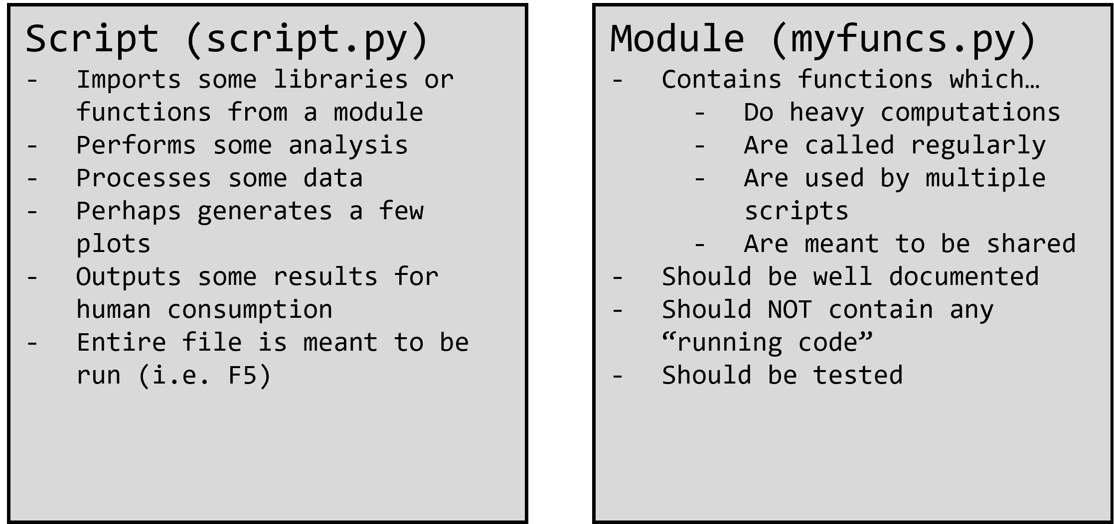
A script is a .py file which we create in our preferred IDE to solve a problem.
A module is a .py file which we maintain in our collection of files that contains helpful functions which we use repeatedly for many problems.
A library (or package) is a collection of several .py files which contain many functions and are categorized for easier access (e.g. numpy.linalg.solve, numpy.random.choice). We can write our own libraries, but usually we will use ones that already exist (e.g. pandas, numpy, scipy, matplotlib, etc.)
Now let’s take a look at this in action. First, let’s create a module which has 2 functions: one for taking the square root of every element in a list, and one for squaring each element.
def square_it(collection):
    for i, val in enumerate(collection):
        collection[i] = val**2
    return collection


def root_it(collection):
    for i, val in enumerate(collection):
        collection[i] = val**0.5
    return collection
The above code should be placed in a new file called something like “myfuncs.py”, as shown below:
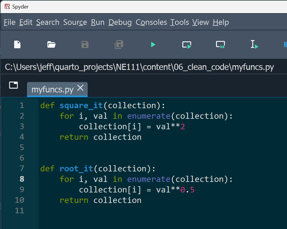
myfuncs.py file containing our custom functions
We can then use the functions in this module in a script as follows:
from myfuncs import root_it, square_it

vals = [1, 3, 5, 9]
squares = square_it(vals)
And the script would look like this:
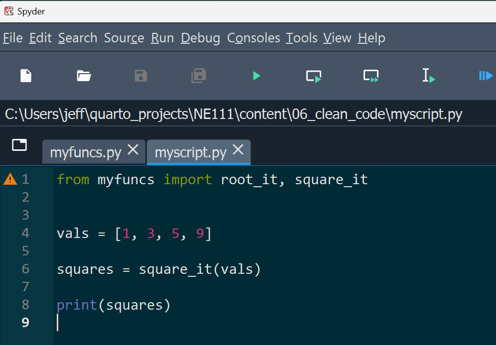
myscript.py showing some calculations using the functions in myfuncs.py
if __name__ == "__main__" to Test Your ModuleIt is as important to test our code as it is to write it in the first place. In fact, in large important projects, more time is spend writing tests than writing code.
Like everything, there are many ways we can do tests, from simple (a script) to complicated (unit testing suites that are run by continuous integration services!).
We probably want the tests to exist closely with the code, ideally in the same file. However, we don’t want a bunch of tests to run each time we import the functions. As usual, Python has a solution for us: The if __name__ == "__main__" block.
Let’s update our myfunc.py file:
def square_it(collection):
    for i, val in enumerate(collection):
        collection[i] = val**2
    return collection


def root_it(collection):
    for i, val in enumerate(collection):
        collection[i] = val**0.5
    return collection


1if __name__ == "__main__":
    # The code inside this "if block" is ONLY executed
    # when you "run" this file. It is NOT run when you
    # import the functions from this file in a script
2    vals = [1, 2, 3]
3    ans = [1, 4, 9]
4    test = square_it(vals)
5    print(test == ans)

    vals = [1, 4, 9]
    ans = [1, 2, 3]
    test = root_it(vals)
print(test == ans)F5). More importantly, this code is not run when the file is imported as a module by another file. This is purely self-contained code, which is a great place to put some rudimentary tests or examples.
True/False, so can visually look at the output and see if anything failed.
True
TrueWith the above if __name__ == "__main__" block added to our module file we can run (F5) the file each time we make changes to the code to ensure our changes didn’t break anything!
We can add as many tests as we want/need to check all the “edge cases”.
It is not necessary to a “unit test suite” for a small personal project, but it is worth knowing what unit tests are, and roughly how they work.
A “unit test” is a function that tests one single aspect of your code, or a single ‘unit’. A unit test might look as follows:
test_, which is the common convention for tests.assert. This is meant for testing purposes, and it will cause an Error if test is not equal to the expected ans. As we saw above, we can catch Errors and deal with them, which is what “testing packages” do. If they detect an error, then collect it, then report them all at the end of testing.
We can then include several of these “unit tests” in a single file (mytests.py) as follows:

mytests.py file which imports our functions from myfuncs and contains several “unit test” functions, indicated by the test_ prefix.
unittest vs pytest
Although Python include a unittest package in its standard library, there is another package called pytest, that is more widely used. This package is used by everybody and has many, many features. It even supports a plug-in system so that extra functionality can be added. Here is a detailed tutorial on RealPython. And here is a video introduction to pytest specifically.
And we can “run” all these tests using a command-line. For this demo we will use pytest. To have pytest test our package we do the following:
mytests.py)python -m pytest mytests.py and hit enter
pytest after running all the tests it found in the mytests.py file
Here is what things look like when a test fails:
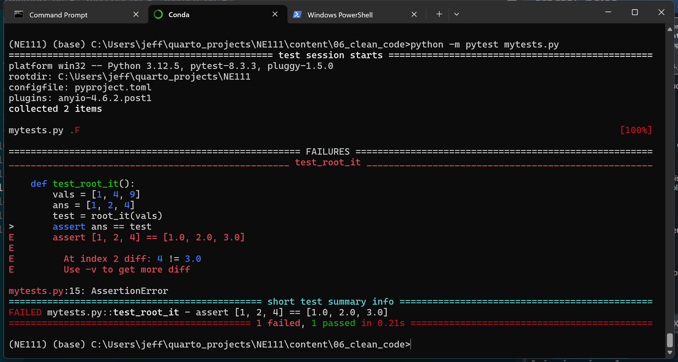
pytest when one or more tests fail
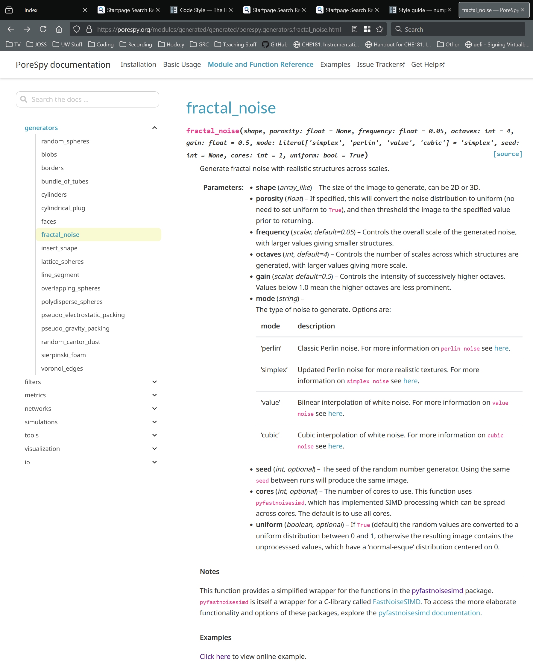
Large projects contain a LOT of tests. My lab group maintains a package called PoreSpy, which is hosted on GitHub. Each time we write new code and “push it” to GitHub, a set of unit tests is automatically run. Below is the output:
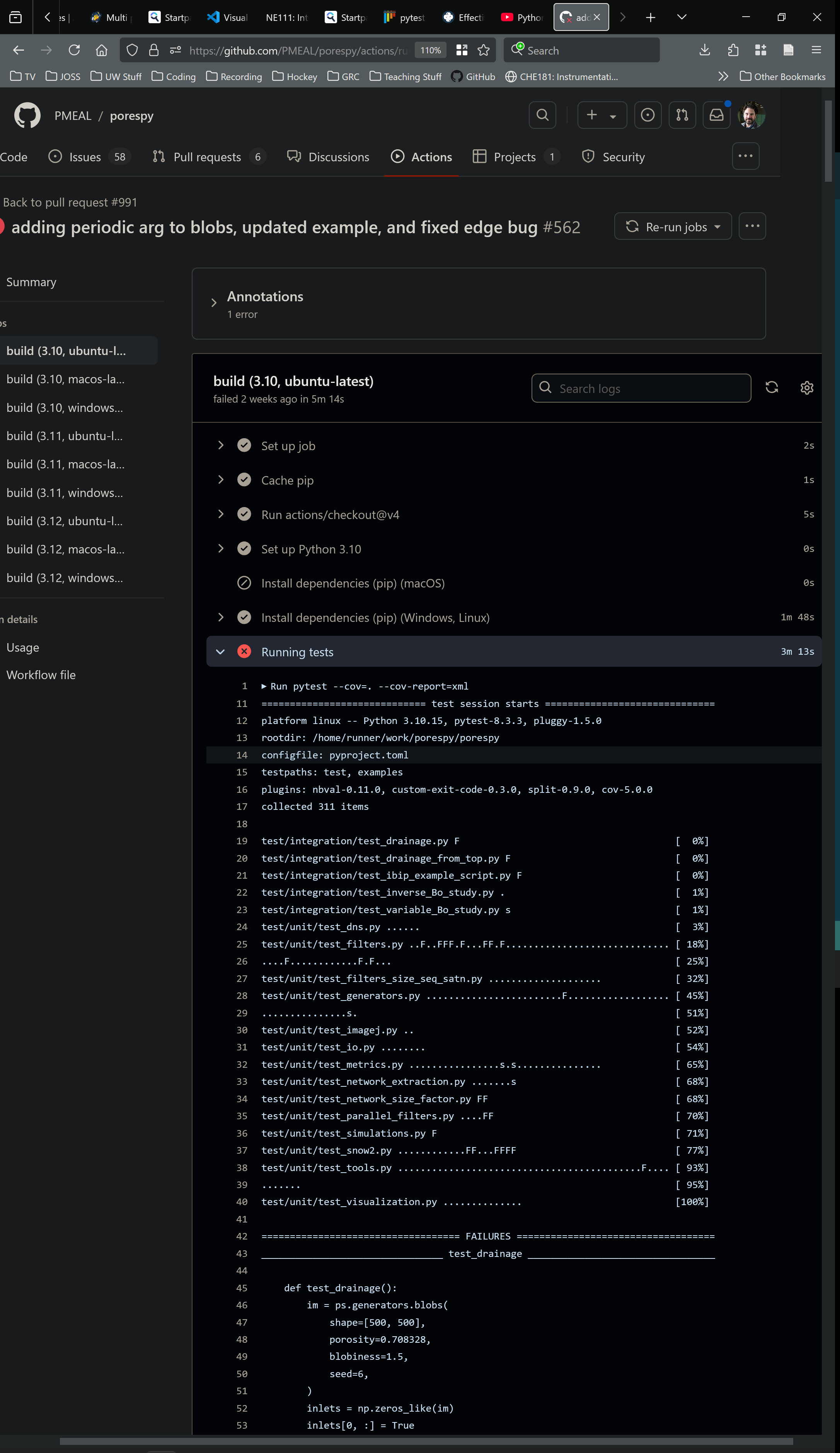
pytest on PoreSpy. There were 311 tests, and unfortunately quite a few of them failed (as indicated by the “F”s), so this changes made by this code broke quite a few tests. We’ll have to do quite a bit of work to get this code ready for inclusion in PoreSpy.