2 Introduction to Programming (with Python)

Learning Outcomes for this Lesson

Upon completion of this lesson you should:

…fully accept that learning Python is very important for your success as an engineer
…be well versed the basic syntax of Python expressions, like the meaning of * and /
…know how to write simple mathematical expressions incorporating order of operations
…have installed Python and used both Jupyter and Spyder IDE to run some code snippets
…know how to assign values to variables and use them in subsequent expressions
…have used Python’s built-in functions
…know how to import functions from Python’s standard library
…be able to define your own custom functions

2.2 Motivating Examples

2.2.1 Computers Are OP calculators

What are the tools you associate most closely with the job of “engineer”? Probably a calculator!

Example 2.1 (Using Python as a calculator with units) If an object is traveling 1,000 furlongs every half a fortnight, what is its velocity in SI units (m/s)?

Solution

import pint
u = pint.UnitRegistry()

a = 1000*u.furlongs
b = 0.5*u.fortnight
c = a/b
print(f"The velocity of the object is {c}")
c.ito_base_units()
print(f"The velocity in SI units is {c}")
print(f"The velocity with better formatting {format(round(c, 3), '~')}")

The velocity of the object is 2000.0 furlong / fortnight
The velocity in SI units is 0.3326197128584733 meter / second
The velocity with better formatting 0.333 m / s

Comments

We will “unpack” all of the steps over the next few weeks, but hopefully you can appreciate the value of using Python for doing homework assignments in courses other that this one.

Syntax highlighting

Throughout these notes (and the internet in general) you’ll see computer programs (often referred to as “code”) written in the following format:

1# This is a comment
2a = int(1.0)
3b = 'some text'
4print(b)

1: Outside a string, # starts a comment that continues to the end of the line and is ignored by Python
2: Numbers are given a special color so they stand out. The color scheme is called “syntax highlighting” and helps programmers recognize features of the text (i.e. numbers and text are different colors).
3: You’ll also usually see “code” written using a monospace font that looks like an antique typewriter.
4: In this code block the print() statement is actually run and the output is printed below.

some text

Also, the grey background is used to indicate a code block. And you’ll notice an icon in the top-right corner, which will “copy” the contents of the block so you can paste it into your own program.

2.2.2 Computers Are Crazy Fast

Have you ever had to do an extremely boring but repetitive task? Computers were literally invented to solve that problem!

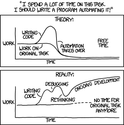
Figure 2.3: The dream vs. the (sad) reality of writing programs that make our lives easier. One unstated takeaway from this joke is that writing the program can actually e quite fun and satisfying.

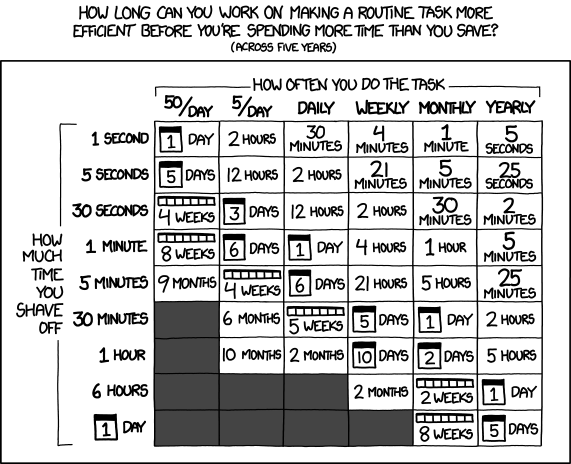
Figure 2.4: How to decide if it’s worth your time to automate a task (assuming the situation in Figure 2.3 does not occur!)

Example 2.2 (Using Python to fix mailing addresses) You have used Google Forms to collect mailing addresses of people, and now you wish to send them a letter. You realize, however, that the output of Google Forms looks like this:

Name	Street and Number	City	Province	Postal Code
Mr Jimmy Beast	100 Main St	Toronto	Ontario	M2T1T2
Ms Taylor Swift	999 Bay St	Topeka	Kansas	90210

But we need them to look like the following so we can print them onto the envelopes:

Mr Jimmy Beast
100 Main St
Toronto Ontario
M2T1T2

Solution

text = "Mr Jimmy Beast, 100 Main St, Toronto  Ontario, M2T1T2"
text = text.replace(', ', '\n')
print(text)

Mr Jimmy Beast
100 Main St
Toronto  Ontario
M2T1T2

Comments

If we had a list of hundreds or thousands of addresses, the computer could zip through them all in milliseconds (or less!).

2.2.3 Making Beautiful Data Dashboards

Many non-technical people still have to deal with data, so they will seek help from engineers (such as yourselves). There are many tools to help us make ‘user-interfaces’ so normies can interact with a computer. Even Facebook is arguably just a web-based user interface for a social network graph.

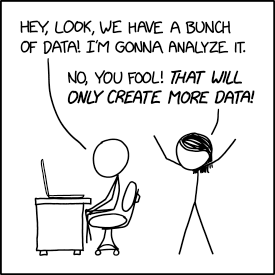
Figure 2.5: Not everyone loves data as much as engineers.

Example 2.3 (Develop a graphical user interface for simulating a hydrogen fuel cell) There are many, many frameworks available for making graphical interfaces so users can interact with a computer program. Some are extremely powerful but hard to use, while others offer basic features but are super easy. Streamlit is one of my favorites. It is very fast to learn, requires only pure Python, and renders in the web browser.

Solution

Comments

You can play with this app here.

Good news: you will be using Streamlit to make your own app for the project in this course!

2.3 Getting Started with Python

“To begin, begin” - William Wordsworth

2.3.1 Your Programming Environment

Using Python requires using a lot of different pieces of software. It is helpful to understand the relationship between all these pieces. Figure 2.6 shows the relationship between you and your computer, the programming environment which exists on your computer, and the internet where all the software we use is stored.

The programming environment is a subset of your computer as a whole, which is used for many other purposes.
The Anaconda installer is a useful way to get everything installed all at once
It is possible to get all the pieces individually but it takes some experience/expertise (which you’ll gain soon!)
IDEs are a useful way to communicate with Python, instead of just typing code at the Python prompt. IDEs let you collect your code in files so you build up complicated “scripts”. They provide convenience features like “help” and “autocomplete”.
Python can be extended by installing “packages” like Numpy and Scipy (which we’ll cover in Chapter 8)

Figure 2.6: This diagram attempts to illustrate the relationship between yourself, your programming environment on your computer, and the internet.

2.3.2 Installing Python

There are many ways of installing Python. One can:

download the official installer
install a standalone editor distribution that bundles a Python environment, such as the Spyder standalone installer
install VS Code and its Python extension, then install and select a Python interpreter; the extension itself is not the interpreter
install uv to manage Python versions and install packages from PyPI

For our purposes, we will do the following:

Install the Anaconda distribution of Python, which is a convenient way to get our ‘coding environment’ setup all at once as illustrated in Figure 2.6
Open the “Anaconda Navigator”
Launch Spyder

Figure 2.7: Screenshot of the Anaconda Navigator showing several items including Spyder

2.3.3 Using Jupyter Notebooks

Video: Jupyter notebooks

Michael Fudge · about 7 min. See how notebook cells combine Python code, output, and Markdown, and how to run cells interactively.

Watch on YouTube.

The name Jupyter

Jupyter notebooks grew out of IPython Notebooks, where the “I” stood for “interactive”. Jupyter supports different programming languages through language-specific kernels. Its name refers to Julia, Python, and R, three languages used for numerical computation. Many other kernels are available too.

Note that notebooks still have the .ipynb file extension regardless of which language was used within it.

Jupyter Notebooks offer the following two benefits:

You can mix programming-related information like code, outputs, and graphs with text-based information like headings, explanations, and equations.
Once a notebook is complete you can save it to a permanent format like a PDF file to be shared like a normal document.

So basically, Notebooks are a way to share the results of our computations with others. They have become a popular way for programmers (such as ourselves) to do quick calculations because they make it easy for us to remember what we did and why (assuming we included good explanations!).

To launch the Jupyter environment, you can do either:

Open Anaconda Navigator and click “Launch”
Open the (Ana)conda prompt, and type jupyter notebook

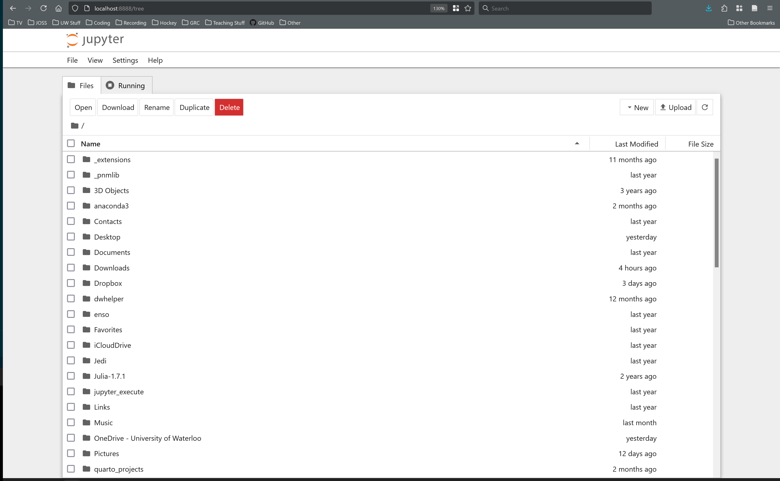
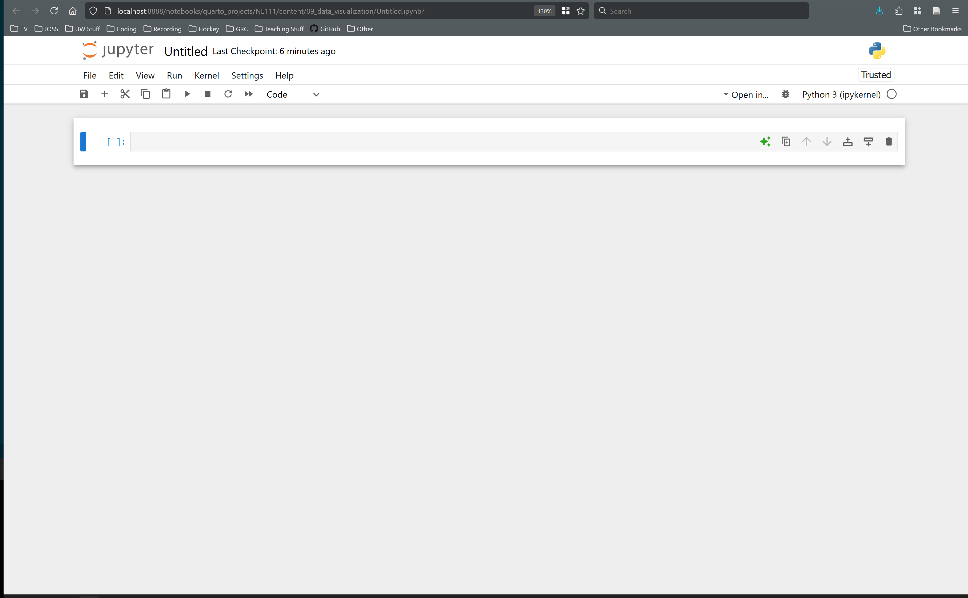
You will end up seeing something like the following in your web-browser:

Figure 2.8: Left shows the file browser and right shows the notebook itself.

Notebooks are based on the concepts of “cells”.

Each notebook is a linear series of cells
Cells can contain either text or code
The output of code cells is rendered immediately below the cell
Text cell can be formatted with a syntax called Markdown
Text cells can also contain equations written using Latex syntax

Jupyter shortcut keys

When working with any program it is extremely useful to learn the shortcut keys. A list of shortcut keys for Jupyter is given in Appendix B.

The process for running Python code in a Jupyter notebook is:

Press enter to begin editing a cell
Enter the Python commands using your keyboard
Press ctrl/cmd-enter to run the cell

You can enter text into a cell by entering Markdown mode:

Press Escape to enter command mode, then m to change the cell to Markdown
Press enter to begin typing text into the cell
Press ctrl/cmd-enter render the contents of the cell

Example 2.4 Use a Jupyter notebook to determine the sum of 123 and 345.

2.3.4 Using Spyder

Spyder is called an “Integrated Development Environment” or IDE. This means it is a single piece of software (an Environment) used for doing computer programming (Development) that includes a text editor, documentation, terminal, and other helpful features all in one place (Integrated).

As shown in Figure 2.9, Spyder lives in the sweet-spot for ease of use and utility. More importantly, Spyder is optimized for numerical computing. VSCode is great if you code using 5 different languages on a daily basis, and PyCharm is great if you do many different tasks in Python like Django websites, SQL databases, etc.

Figure 2.9: A comparison of “Integrated Development Environments” (IDEs)

When we open Spyder we will see the following:

Figure 2.10: The default layout of Spyder is a text editor, help panel, and a Python console. Each is exceedingly useful and any coding environment which does not supply all three simultaneously makes things harder than necessary.

Figure 2.11: This screenshot shows Spyder with a dark color scheme, which is *much* easier on the eyes during long programming sessions.

The workflow for programming in Spyder is as follows:

Write some python “code” in the “editor” window on the left
Run the code by pressing F5 or clicking the “Play button” (green arrow)
Move to the “console” to explore the data and check values (see Note 2.1)
Switch back to the editor, update code, and repeat

Example 2.5 Using Spyder, determine the sum of 123 and 345 by working directly at the console, then again by entering the commands into the text editor and running the file.

Note 2.1: The REPL: One of Python’s superpowers

The python console is interactive. The general term for this type of console is a REPL, which stands for “Read-Evaluate-Print-Loop”. It provides a very powerful way to explore data and develop code. The value of this is not really obvious until you don’t have it.

When you run a file (i.e press F5) all the data and variables are available in the REPL, so you can explore them (i.e. how big is my array?). You can also write snippets of code in the REPL to see if they’ll work, then copy-paste them into your file for permanent usage. In other words, if you reboot your computer the data in the REPL session will be gone, but the text in the file will remain (assuming you saved the file).

Two kinds of Python consoles

The standard Python console is indicated by three >>>. It is technically a REPL, but has very few features like “autocomplete”.

>>> print('hello world')
hello world

There is also the IPython console which stands for “Interactive Python”. This is indicated by In [1]:

In [1]: print('hello world')
hello world

These are different interfaces to Python; each console uses the interpreter selected for its environment. Spyder uses IPython for its handy features, including my favorite shortcut (Note 2.2).

An assignment such as x = 2 stores a value without displaying it. Entering x at the console, or as the last expression in a notebook cell, displays its value. In a script, use print(x) to produce output. print() writes text and returns None, so its printed text has no Out[...] label. Editing a cell does not update its variables until you run it again; restart the kernel and run all cells in order to check that a notebook works from a fresh session.

When using any piece of software it is essential to learn its keyboard shortcuts. For example, in Windows you can use ctrl-c/x/v to copy/cut/paste text (it’s cmd-c/x/v). If you’re not using these you’re wasting a lot of time!. IDEs have a lot of extra shortcuts to help coders be more productive. Table 2.1 shows a small subset of the common shortcuts in Spyder.

Table 2.1: A sample of Spyder’s default shortcuts on Windows/Linux, with the macOS run-cell shortcut noted. Shortcuts depend on the focused pane and can be customized under Preferences → Keyboard shortcuts. See the Spyder code-cell documentation.

Key or Character	Result
`F5`	Runs an entire file, putting result in console
`F9`	Runs current line or highlighted selection
`# %%`	Creates a new cell in a file
`Ctrl-Enter`	Runs current cell (`Cmd-Return` on macOS)
`Shift-Enter`	Runs current cell and advances to the next one
`Ctrl-Up Arrow`	Moves cursor to preceding cell
`Ctrl-Down Arrow`	Moves cursor to next cell
`Ctrl-L`	Clears the IPython console when it has focus
`Alt-Up/Down Arrow`	Moves current line up/down
`Ctrl-Alt-Up/Down`	Duplicates current line up/down
`Tab or Ctrl-Space`	Open “Suggested Completions”
`Ctrl-i`	Open documentation for selected item

2.3.5 The Basic Syntax of Python

Video: Arithmetic in Python

Socratica · about 5 min. Review arithmetic with integers, floats, and complex numbers, including how division works in Python 3.

Watch on YouTube.

First let’s look at mathematics, since this is one of the most common uses of Python for engineers. In “real” mathematics we use symbols like $\times$ and $\div$, but we do not have these on our keyboard, so we had to improvise. The following table lists the keys for each mathematical operation.

Table 2.2: List of mathematical operations and corresponding keyboard symbols. Use ** for exponentiation: ^ performs bitwise exclusive OR on integers, so 2 ^ 5 gives 7, not 32. With floats, ^ raises a TypeError.

Symbol	Operator	Example Expression	Resulting Value
`-`	negation	-5	-5
`+`	addition	11 + 3.1	14.1
`-`	subtraction	5 - 19	-14
`*`	multiplication	8.5 * 4	34.0
`/`	division	11 / 2	5.5
`**`	exponentiation	2 ** 5	32
`//`	floor division	11 // 2	5
`%`	remainder	8.5 % 3.5	1.5

Square root sign?

What about the famous $\sqrt 2$ sign you ask? We will have to remember our high school math rules and use 2**0.5.

Below are some snapshots of these operators in action:

11 + 3

11.4944 + 3.0002

14.4946

5 - 9

-4

10/2

5.0

2**16

2**-0.5

0.7071067811865476

But we will do a lot more with Python than just math. Many keyboard symbols have special meanings in Python. Below is an introductory summary:

Table 2.3: Nearly exhaustive list of characters used in Python and what they do. Don’t worry, you don’t have to remember these all at first glance.

Symbol	Name	Use(s)
`.`	Period	The normal decimal point, namespace demarcation
`,`	Comma	Used to separate items in a list…not like 1,000,000!
`_`	Underscore	Used in names; separates digits in numbers like `1_000`
`<`, `>`	Angled Brackets	“Less than” and “greater than”
`=`	Equal Sign	Used for variable assignment…not equivalency!!
`==`	Double Equal	Used to check if two things are equivalent
`!=`	Exclamation Mark	Used to check if two things are not equivalent
`*`	Asterisk	Multiplication, arg unpacking
`**`	Double Asterisk	Exponentiation, kwarg unpacking
`+`	Plus Sign	Addition, concatenation (joining things)
`-`	Minus Sign	Subtraction
`%`	Percent Sign	Modulo (remainder)
`//`	Double Slash	Floor division
`/`	Forward Slash	Normal Division
`( )`	Round Brackets	Groups expressions, encloses call arguments or tuples
`[ ]`	Square Brackets	Indicates a `list`, used for indexing into containers
`{ }`	Curly Braces	Indicates a `dict` or a `set`
`:`	Colon	Introduces a block after headers such as `if`/`for`; also used in slices and dictionaries
`#`	Hash Tag	Outside a string, starts a comment through the end of the line
`\`	Backslash	Line continuation or escape character within text
`@`	“At” Symbol	An operator for matrix multiplication (`b=A@x`)
`~`	Tilde	Integer bitwise complement: `~x == -x - 1`, so `~1001 == -1002`
`'`, `"`	Single, Double Quotes	Used to denote a string of letters
`&`	Ampersand	Bitwise AND on integers; use `and` for logical conditions
\|	Pipe	Bitwise OR on integers; use `or` for logical conditions
`^`	Caret	Bitwise exclusive OR on integers
`;`	Semicolon	Separates simple statements on the same line
`?`	Question Mark	Not Python syntax; IPython uses it for help, e.g. `len?`
`$`	Dollar Sign	This one is actually unused, but is not always present
`	Back Tick	This one is also unused

Some operators have additional meanings for other types. We will revisit & and | with sets and with NumPy arrays in Chapter 8. In IPython, a trailing semicolon can suppress the automatic display of an expression’s value, but it does not suppress text written by print().

2.3.6 Introduction to Data Types

We will introduce data types more thoroughly in the next chapter, but there is an important point to be made here: there is a difference between 1 and 1.0, and "1".

1 is an integer literal, so its Python type is int. Adding or multiplying integers produces another integer, such as 1 + 3, which gives 4. For mixed int/float addition or multiplication, Python converts the integer operand to a float for that operation. For example, 1 + 2 + 3.0 gives 6.0.
1.0 is a floating-point literal, so its type is float, even though its mathematical value is a whole number. Exponent notation such as 1e3 also creates a float. Floats represent numbers with finite precision: many decimal fractions, such as 0.1, cannot be represented exactly in binary. Converting an integer to a float can also lose precision if the integer is large enough. The / operator on integers or floats produces a float, as in 1 / 2, which gives 0.5.
"1" is not even a number, it’s just the text for the number 1. This data type is called a “string” (as in string of characters) or str in Python. Obviously if we attempt to do math with the character "1" Python will not do what we want. In fact, if we attempt to multiply "1" by 2, Python will give us "11", which actually makes some sense if you think about it.

This last example is perhaps the best demonstration of why data type matters: So Python “knows” how to handle operations on each variable.

2.3.7 Operator Precedence (aka Order of Operations)

Operator precedence in Python is based upon the same concepts used in actual math:

Table 2.4: Order of operations for mathematical statements. NOTE: Operators of equal precedence are applied from left to right except exponentiation, which is applied from right to left.

Precedence	Operator	Operation
1 (highest)	`**`	exponentiation
2	`-`	negation
3	`*`, `/`, `//`, `%`	multiplication, division, floor division, remainder
4 (lowest)	`+`, `-`	addition, subtraction

Using these precedence rules, operators of higher precedence are evaluated before those with lower precedence. In order to specific a desired order of evaluation we may use parentheses or round brackets: ().

Example 2.6 (Experiment with various forms of division) Paste the following code into a blank file in Spyder. Try running the entire file, each cell, and each individual line. A bare expression can display its result when evaluated interactively, but does not print when run as part of a script. To see each result when running the entire file, wrap each expression in print(...), for example print(9 / 2).

# %%
9 - 3

# %%
8 * 2.5

# %%
9 / 2

# %%
9 / -2

# %%
9 // 2

# %%
9 % 2

# %%
9.0 % 2

# %%
9 % 2.0

# %%
9 / -2.0

# %%
4 + 3 * 5

# %%
(4 + 3) * 5

Solution

Let’s run all of these in a Jupyter Notebook for practice. The answers will be as follows:

9 - 3

8 * 2.5

20.0

9 / 2

4.5

9 / -2

-4.5

9 // 2

9 % 2

9.0 % 2

1.0

9 % 2.0

1.0

9 / -2.0

-4.5

4 + 3 * 5

(4 + 3) * 5

Comments

There are few common behaviors we can identify:

Mixed int/float arithmetic in these examples produces a float. This does not guarantee an exact result: floating-point representation has limited precision.
/ applied to integers or floats produces a float, even when the result is a whole number. // instead rounds the quotient down toward negative infinity. It returns an integer when both operands are integers, and a float when either operand is a float.

Compare floor division with conversion to int, which truncates toward zero:

print(-9 // 2)    # -5: round down
print(int(-9/2))  # -4: truncate toward zero
print(9.0 // 2)   # 4.0: a float operand gives a float result

-5
-4
4.0

Note 2.2: My favorite Spyder shortcut

When your cursor is in the terminal, you can press the up arrow to scroll previous commands. This is normal at most terminals. Spyder offers an extra feature: if you type a letter (i.e. p) the press the up arrow it will only show you previous commands that started with p. This is a massive time saver for repeatedly calling something like a plot command.

2.3.8 Item Assignment

Video: Variables and assignment

Programming with Mosh · about 7 min. Learn how to assign values to names and use variables holding numbers, strings, and Boolean values.

Watch on YouTube.

So far we have used Python like a dumb calculator that just prints out an answer. It becomes a lot more useful once we store the result of each calculation for later use. For instance:

a = 9
b = 2
c = a / b
print(c)

4.5

= does not mean equal!

The main thing to note here is that = sign does not mean “equals”! It is better to think of it as gets, as in a gets 9. Or is assigned as in a is assigned 9. As we will see in Section 4.1, equality is checked with ==.

So if you see x = x + 5 it does not mean that the world has gone mad.
For an integer x, x == (x + 5) is False: this compares two values instead of changing x. We’ll look at relational operators in a few chapters.

For comparison, the language R avoids this confusion by using arrows to denote the assignment of values like:

# R assignment syntax, not Python assignment
x <- 1.0

which very clearly means that the value of 1.0 is being written to the variable x. Interestingly, this notation allows things to work in both directions too, like:

# R assignment syntax, not Python assignment
1.0 -> x

In Python, x <- 1.0 is parsed as the comparison x < -1.0, not assignment. Python also uses -> in function return annotations. Use = to assign values in Python.

Another example of storing items in variables is for declaring constants:

1T = 298.0
# Lots of lines here
2P = n*R*T/V

1: We assign the temperature to T at the top of the file where it’s easy to find
2: And we can use T to get the pressure P. Of course we must not overwrite T before step 2!

An interesting conundrum occurs when we wish to swap values between two variables:

A = 4
B = 10
temp = A
A = B
B = temp
print("The value of A is now:", A)
print("The value of B is now:", B)

The value of A is now: 10
The value of B is now: 4

This approach uses a temporary variable to preserve the original value of A before overwriting it. Think of putting one object down while swapping two objects on a shelf. Python also supports A, B = B, A, which swaps the values without an explicit temporary variable; we will explain this unpacking syntax in Section 3.2.3.

2.3.9 Functions

2.3.9.1 Built-In Functions

Python includes a fairly long list of “built-in” functions, a subset of which are given in Table 2.5. Many of these will be gibberish (for now), but there are a few which we should recognize, such as abs(), round() and pow().

Table 2.5: Subset of the built-in functions in Python and what they do. For the full list see Table A.2

Function	Description
`abs()`	Returns the absolute value of a number
`complex()`	Returns a complex number
`divmod()`	Returns the quotient and the remainder when argument1 is divided by argument2
`float()`	Returns a floating point number
`help()`	Executes the built-in help system
`int()`	Returns an integer number
`pow()`	Returns the value of x to the power of y
`print()`	Prints to the standard output device
`round()`	Rounds a number
`type()`	Returns the type of an object

Example 2.7 (Playing with some built-in functions)

Find the absolute value of -11.3
Round pi to 3 decimal places
Find the value of $2^7$

Solution

print(abs(-11.3))                  # (a)
print(round(3.141592653589793, 3))  # (b)
print(pow(2, 7))                   # (c)

11.3
3.142
128

Comments

There are a lot more functions available to us, but they need to be “imported”. Python only exposes the set that it deems essential. For instance, trigonometric functions are not needed by someone writing a web-scraper, while HTTP requests are not needed by an engineer computing the volume of an object.

2.3.9.2 Importing Functions

Video: Importing modules

Bro Code · about 7 min. Compare import, aliases, and from ... import ..., then see how a module supplies reusable functions.

Watch on YouTube.

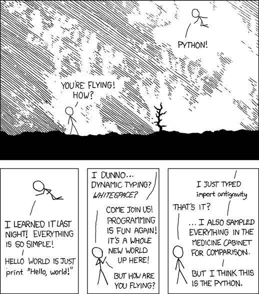
Figure 2.12: The Python Package Index, which is the main place to find new libraries has over 0.5 million packages available for free! Note that the `print "Hello, world"` syntax is Python 2! In Python 3 we write `print("Hello, world")`.

Python itself has a limited set of functions, like those shown in Table A.2. One of the reasons Python is especially useful are the many, many external libraries that have been written for it. In some ways, Python has benefited from the network effect, where people write libraries for Python because it has the most libraries, and so on.

Some packages are used commonly enough that Python includes them within itself. This set of extra packages is called the Standard Library. These packages contain functions which are not core to Python, but are important enough that they are officially supported by the Python team, and are available in every normal Python installation.

A prime example is the math package. It provides a huge variety of extra mathematical functions, essentially turning our standard calculator into a scientific calculator.

Installing packages

The Python Package Index is home to over 0.5 million packages. These are not included in the Standard Library so we need to install them. There are several ways to do this, but they will be discussed later in the course.

Accessing these extra powers is easy:

from math import sin, pi
sin(pi/4)

0.7071067811865475

We can also import the entire math library and then access each of the sub-functions as follows:

import math
1math.sin(math.pi/4)

1: Note the . is used to indicate that you are accessing items below the math library. This is like a . in a section number: 1.2.a, where each indicates a new level of depth.

0.7071067811865475

Namespaces help keep things organized

When we import the math module using import math, we access its functions using qualified names, for example math.tan(0.5). The name math refers to the module, whose namespace contains names such as tan and pi. Keeping each module’s functions under its own name avoids collisions between functions with the same name.

The following will cause a problem:

from math import tan
from colors import tan  # This is not a real package!

While this approach is safe:

import math, colors

# Then we access the respective tan functions as:
math.tan(0.5)
colors.tan()

There is one more useful feature of namespaces: you can choose which namespace you want to import a library as, called an alias:

import math as m

# Now we avoid typing 3 letters:
m.tan(0.5)

The math package has a lot of functions in it. How do you know what functions are available and what they are called? For example, what if you can’t remember if it’s called acos or arccos? Use tab/ctrl-space in Spyder to the autocompletion menu!

Figure 2.13: This screen capture not only shows the ‘autocomplete’ menu, which lists all the available functions in the `math` package, it also shows the help window (for the `acos` function) in the top right.

2.4 Assignment 1: Python expressions in Jupyter notebooks

Submit one Jupyter notebook named A1.ipynb. This assignment is about writing expressions, assigning values to variables, and using basic library functions.

Use one code cell for each question. The first non-blank line in that cell must be the indicated tag, such as # A1Q1. To test your work in Jupyter, you may first assign your own example values to the provided input variables. When the grader runs the cell, it replaces those top-level test-value assignments with its own values. You may include additional variables and print statements if they help you work, but only answer is checked.

If you need imports shared by several questions, place them in a separate code cell whose first non-blank line is # setup. Setup cells are run before each question cell. Do not use notebook magics (such as %matplotlib) or shell commands (such as !pip).

2.4.1 Installing and Using the Checker

The assignment will be graded using an automated systems that runs your notebooks. To ensure that your assignments are formatted properly and the code is correct, you may wish to use the ‘checker’. The instructions for installing and using the checker can be found in Appendix E.

2.4.2 Questions

Question 1: Remainder

The checker provides numbers a and b. Calculate the remainder when a is divided by b and assign it to answer.

# A1Q1
answer =

Question 2: Operator precedence

The checker provides numbers a, b, and c. Calculate the value of $a + b \times c$ and assign it to answer. Use one expression so that Python’s normal operator precedence determines the order of operations.

# A1Q2
answer =

Question 3: Reassign a variable

The checker provides numbers starting_value, scale, and offset. First assign starting_value to a variable named x. Update x by multiplying it by scale, then add offset. Assign the final value of x to answer.

# A1Q3
x = 
answer =

Question 4: Swap two values

The checker provides values x and y. Swap their values, then compute the value of $x^y$ and store the result in answer:

# A1Q4
answer =

Question 5: Convert Celsius to Fahrenheit

The checker provides a temperature in degrees Celsius as celsius. Use $F = \frac{9}{5}C + 32$ to calculate the temperature in Fahrenheit and assign it to answer.

# A1Q5
answer =

Question 6: Use the math library

The checker provides a positive value. Import math, then calculate:

the ceiling of value;
the floor of value; and
the base-10 logarithm of value.

Assign the sum of these three values to answer.

# A1Q6
answer =

Question 7: Calculate an $n^{th}$ root

The checker provides a positive number number and a positive integer root. Calculate the $root^\text{th}$ root of number and assign it to answer.

# A1Q7
answer =

Question 8: Circle area

The checker provides a radius. Calculate the area of a circle with that radius, and assign the value to answer.

# A1Q8
answer =

Question 9: Types and conversion

The checker provides value. Assign the type of value as a str to answer:

# A1Q9
answer =

Question 10: Absolute difference

The checker provides numbers a and b. Calculate the non-negative difference between them and assign it to answer. Use Python’s built-in abs() function.

# A1Q10
answer =

2.1 Why Python?

2.2 Motivating Examples

2.2.1 Computers Are OP calculators

2.2.2 Computers Are Crazy Fast

2.2.3 Making Beautiful Data Dashboards

2.3 Getting Started with Python

2.3.1 Your Programming Environment

2.3.2 Installing Python

2.3.3 Using Jupyter Notebooks

2.3.4 Using Spyder

2.3.5 The Basic Syntax of Python

2.3.6 Introduction to Data Types

2.3.7 Operator Precedence (aka Order of Operations)

2.3.8 Item Assignment

2.3.9 Functions

2.3.9.1 Built-In Functions

2.3.9.2 Importing Functions

2.4 Assignment 1: Python expressions in Jupyter notebooks

2.4.1 Installing and Using the Checker

2.4.2 Questions